
Scaffold Mapping Tools: Using Subject-Specific Vagus (SSV) Scaffolds For Population-Level Analysis
This tutorial shows how to use the Scaffold Mapping Tools to visualize branching patterns of subject-specific vagus scaffolds using the vagus material coordinates.
Vagus material coordinates, also known as vagus coordinates, are defined as a straight line along the vagal trunk, with the origin as the top of the trunk and 1 as the bottom end of the trunk. The branches are defined as lines with the same orientation as when they leave the trunk.
Mapping branches into these coordinates allows branches from different subjects to be visualized along the same trunk geometry, making it easier to locate branch origins or spatial distributions along a length scale between 0 and 1 for systematic quantification of branch behavior.
Any number of subjects can be added to the visualization. For demonstration purposes, this tutorial uses vagus scaffolds derived from two subjects (f009, DOI: 10.26275/un0a-zzdl) and f019, DOI: 10.26275/8ekx-tqxe), from the Feinstein collection (DOI: 10.26275/2vva-qmjw).
By the end of this tutorial, you will learn how to:
- retrieve subject-specific vagus scaffolds from the SPARC Portal;
- map branches onto a common vagus material coordinates; and
- generate qualitative branch distribution visualizations.
Step 1: Create and execute the workflow
Launch MAP Client Mapping Tools from the Start Menu under MAP-Client-mapping-tools vX.Y.Z (X, Y, and Z will be the actual version numbers).
Set up a new workflow named SSV-vagus-coordinates on your Desktop by
creating a new folder on the Desktop named SSV-vagus-coordinates. In MAP Client Mapping Tools, go to File → New Workflow (Ctrl+Shift+N). Select the SSV-vagus-coordinates directory you just created.
To set up the organ inserter workflow, add the following steps to the workflow area and connect them as shown in Figure 1:
- One Retrieve Portal Data steps
- One Argon Viewer step
- One Argon Scene Exporter step
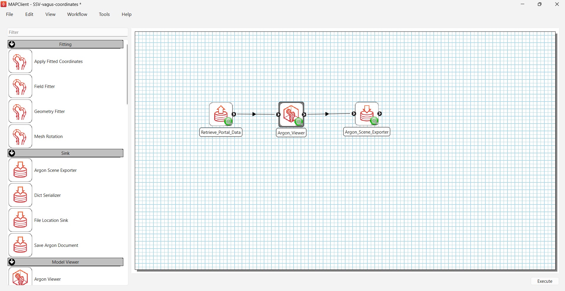
Figure 1. Workflow for visualizing SSV scaffolds in vagus coordinates.
Retrieve Portal Data step
Configure the first Retrieve Portal Data by setting its identifier to SSV scaffolds as shown in Figure 2.
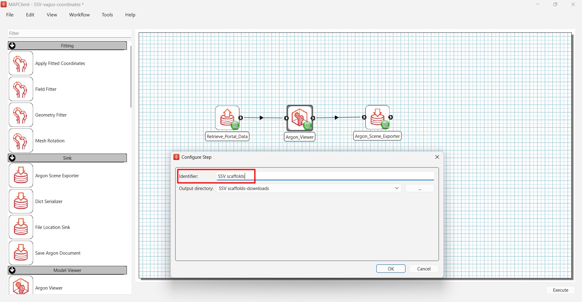
Figure 2. Configuring the Retrieve Portal Data step.
Argon Scene Exporter step
Configure the Argon Scene Exporter step by changing Export type to image, the prefix to branch_directions_left and selecting an output directory for saving the image. Set Width and Height to 2048 in order to export a high-resolution image as shown in Figure 3.
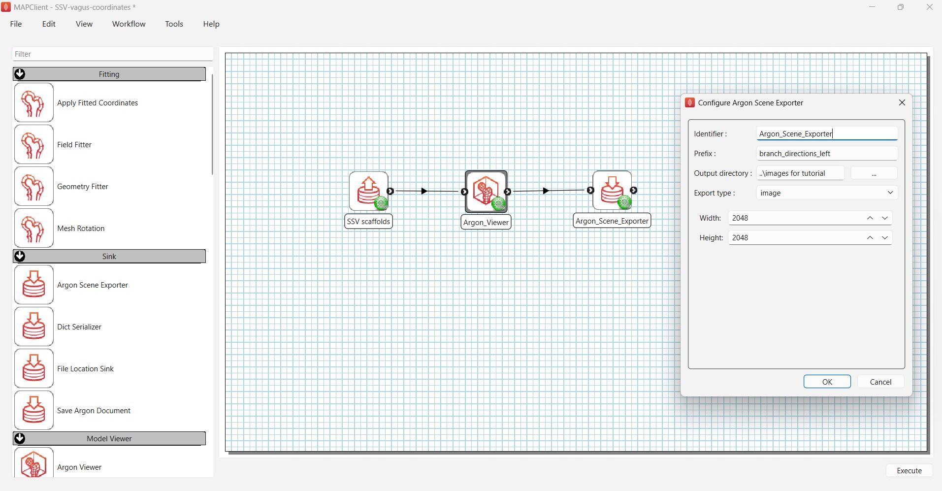
Figure 3. Configuring the Argon Scene Exporter step.
Once the workflow is complete, save it (Ctrl+S) and click Execute.
Step 2: Retrieve data from the SPARC Portal
In this example, we will retrieve the SSV scaffolds for the left side only but the same steps apply to generating visualizations for the right vagus.
Enter https://doi.org/10.26275/tjzi-muqm in the Search term field and click Search. The search results will show up in the Search results panel.
To filter the results to scaffold files, enter scaffold-exf in the Filter field and select Mimetype. Click the Filename header to sort the results alphabetically.
In this example, we are inserting vagus scaffolds from two subjects (f009 and f019). From the list, locate the following two files:f009-left_vagus_scaffold.exf
f019-left_vagus_scaffold.exf
Hold Ctrl while selecting both files, then click Download. Once the selected files are loaded in the Provided files panel as shown in Figure 4, click Done to proceed.
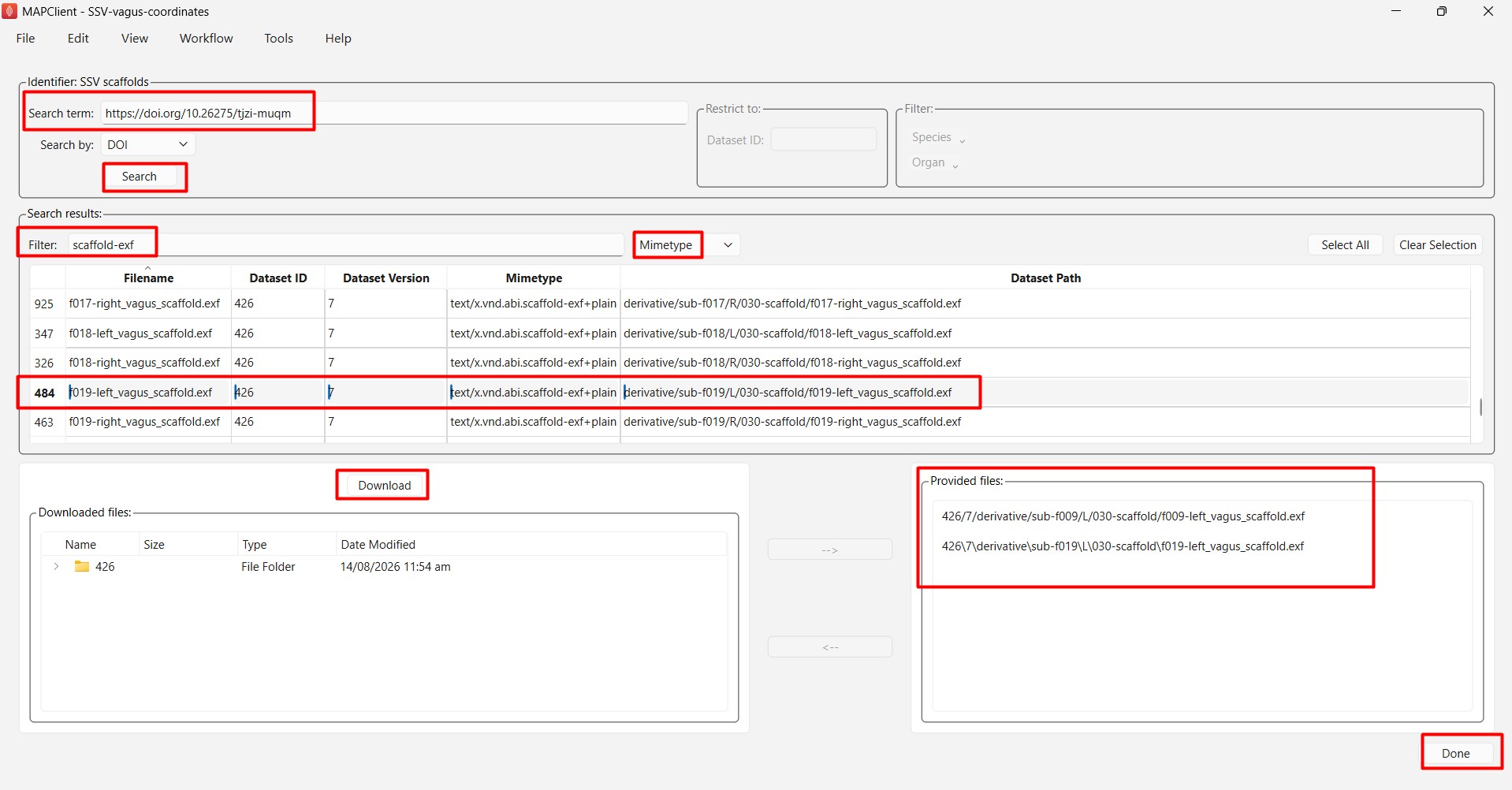
Figure 4. Retrieving and selecting SSV scaffolds.
In the next section, we will use Argon Viewer to visualize the SSV scaffolds in vagus coordinates.
Step 3: Visualize vagus scaffolds with vagus coordinates
Set up view, regions and model sources
Click Add View to add a Layout1 view panel.
Open the Region Editor. Right-click and select Add child region to create two child regions. Double-click each newly created region to rename them f009 and f019. The resulting region hierarchy should look like Figure 5.
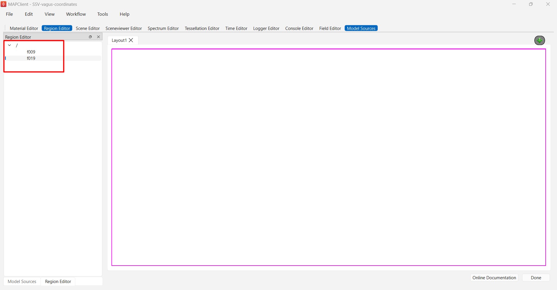
Figure 5. Region hierarchy in Region Editor.
Next, click the Model Sources tab in the top panel. Assign each scaffold file to its corresponding child region by selecting the appropriate region and then clicking the green plus icon, as shown in Figure 6.
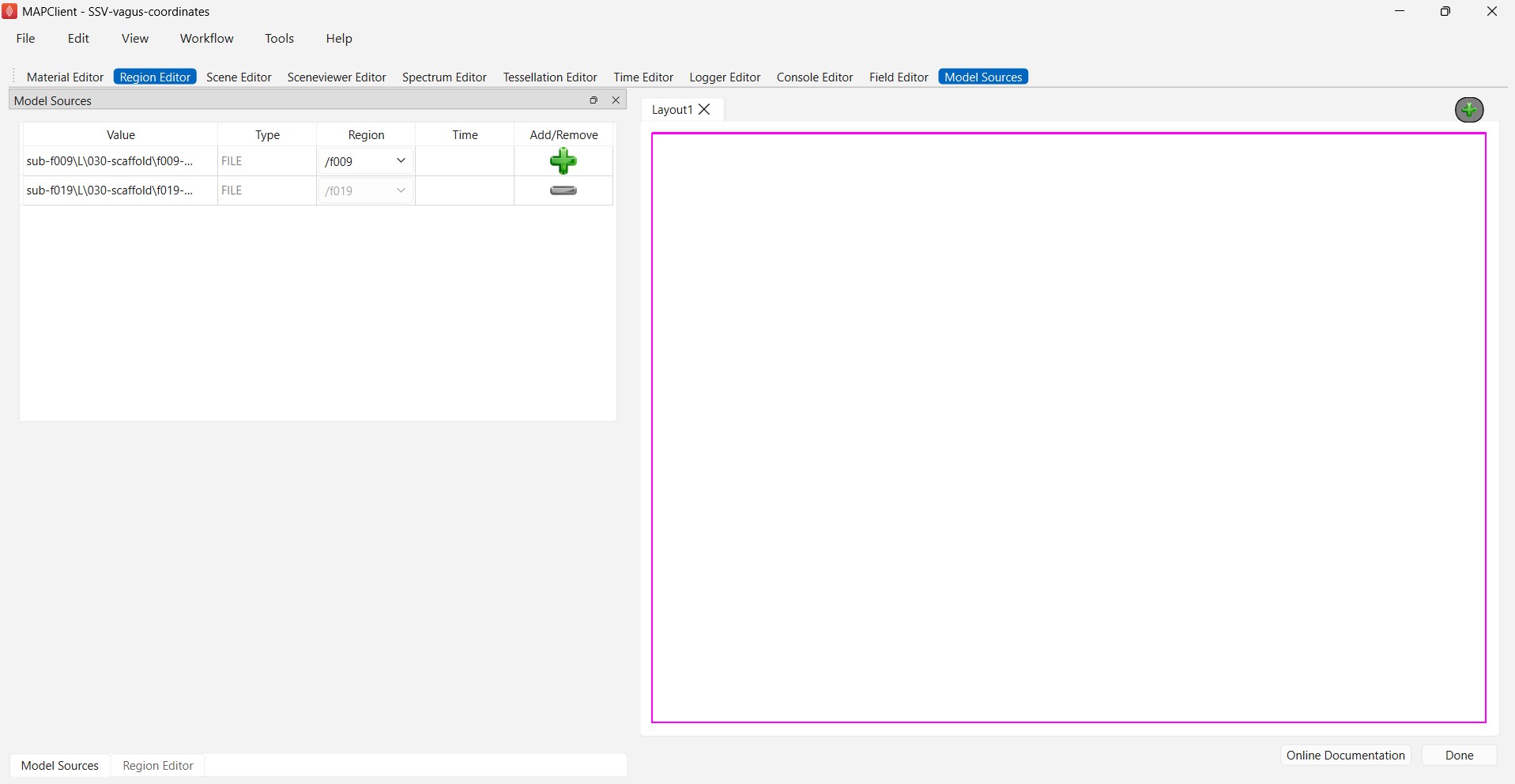
Figure 6. Assigning scaffold files in Model Sources.
Create vagus nerve centroid and normalised branching directions with vagus coordinates
Next, we will set up the vagus trunk centroids. This only needs to be done once per side using any subject, since the trunks from all different subjects should be mapped to the same vagal trunk in the vagus material coordinates. In this tutorial, we will set it up for /f009.
Go to Field Editor and use the following settings to set up a field called left vagus nerve centroid in the Region for /f009 as shown in Figure 7:
Add …: And
Source Field 1: left vagus nerve
Source Field 2: vagus centroid
Name: left vagus nerve centroid
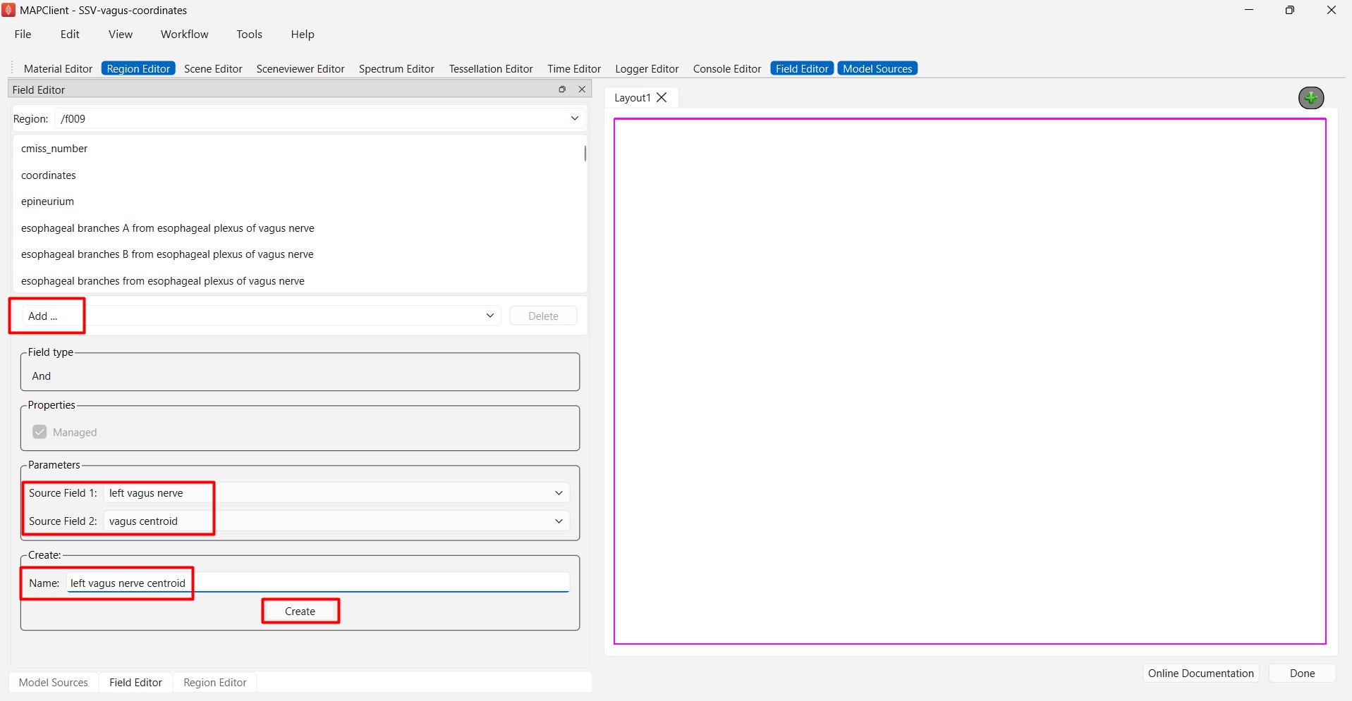
Figure 7. Creating the left vagus nerve centroid field.
As we will be visualizing the origins and initial directions of vagal branches, we first need to create a group called vagus nerve branches.
For each of the vagus sub-regions (/f009 and /f019), create the following field as shown in Figure 8:
Add...: Not
Source Field: left vagus nerve
Name: left vagus nerve branches
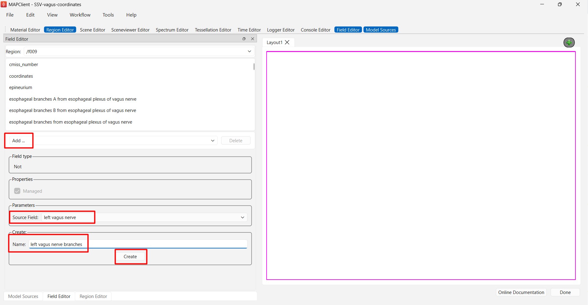
Figure 8. Creating a group for the left vagus nerve branches.
Next, as shown in Figure 9, we add a Derivative field for the same regions with the following settings:
Coordinate Field: vagus coordinates
xi index: 1
Name: vc_dx_dxi1
As the derivative of the coordinates field with respect to the first element coordinates (xi1) provides a vector tangent to the branch, the vector vc_dx_dxi1 represents the local direction of the branch in the vagus coordinate system.
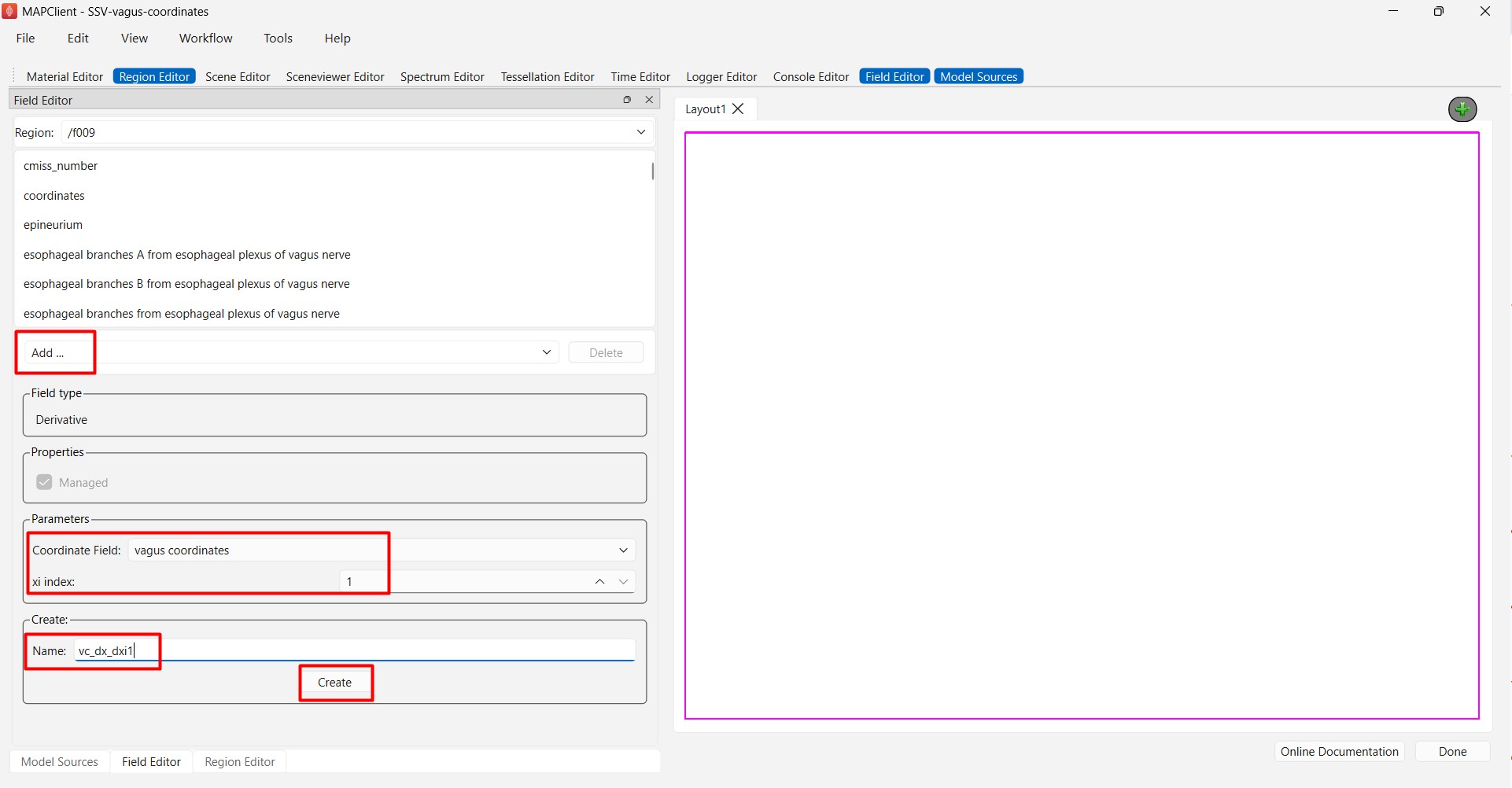
Figure 9. Creating a derivative field representing the branch direction.
Then, we add a Normalise field as shown in Figure 10 for each of the vagus regions:
Source Field: vc_dx_dxi1
Name: norm_vc_dx_dxi1
Normalising vc_dx_dxi1 removes its magnitude while retaining its direction. This allows it to be used to orient the glyphs later for visualization.
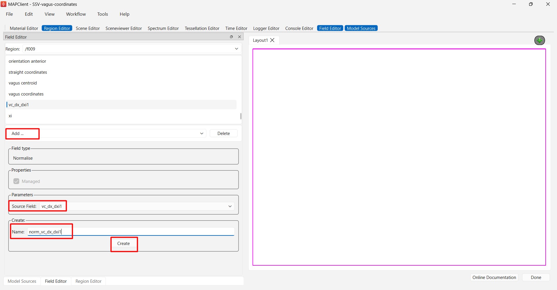
Figure 10. Creating a normalised derivative field representing the branch direction.
Visualize branches using vagus coordinates
Visualize vagus trunk in vagus coordinates
Go to Scene Editor, and for /f009 region, add lines with the following settings:
Subgroup: left vagus nerve centroid
Coordinates: vagus coordinates
Shape: circle extrusion
Base size: 0.01*0.01
At this stage, the Layout1 panel will still be empty. To display the graphics you have just created, open Sceneviewer Editor and click View All. Adjust the graphics to a comfortable viewing position using left-click to rotate, middle-click to pan and right-click to zoom. From this point onward, any newly added graphic objects should appear in the view panel when they are configured correctly.
If you would like to visualize the level markers in the vagus coordinates, add node points with the following settings:
Subgroup: marker
Coordinates: marker vagus coordinates
Glyph: line
Base size: 0.5*0.5*0.5
Label field: marker_name
Glyph offset: -0.5, 0, 0
Label text offset: -0.1, 0.0, 0.0
Visualize branch groups
It is often helpful to create translucent materials when visualizing multiple branch groups, as it makes it easier to see how different groups of branches interact with and overlap one another.
Go to Material Editor, and click Create. Double-click the new material and rename it to magenta50. Select magenta for both Ambient Colour and Diffuse Colour. Then set:
Alpha: 0.5
Shininess: 0.2
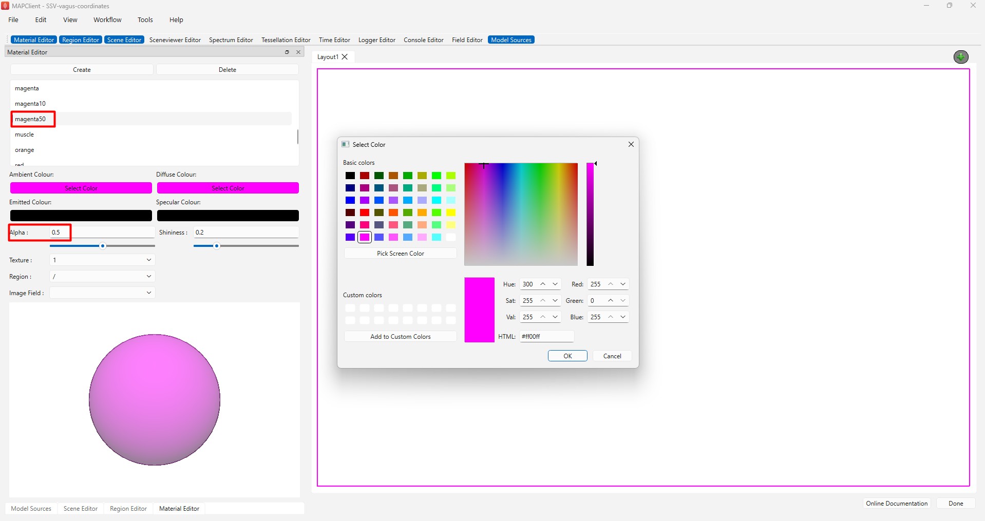
Figure 11. Creating a magenta50 material in Material Editor.
Follow the same steps to create green50, which is a translucent version of the green material.
Go to /f009 region and add element points to visualize the left superior laryngeal nerve with the following settings:
Subgroup: left superior laryngeal nerve
Coordinates: vagus coordinates
Material: magenta50
Glyph: cylinder
Base size: 0.1*0.01*0.01
Scale field: norm_vc_dx_dxi1
Scaling: 0.01*0.01*0.01
Repeat these steps for /f019. You should now be able to see the left superior laryngeal nerves from both f009 and f019 mapped onto the same vagus material coordinates.
We recommend using a translucent material, such as magenta50, to make it easier to identify overlapping branches. Additional vagal branch groups can also be visualized using different materials. For example, the left cardiovascular branch of cervical vagus nerve can be added using a different material (green50) to investigate how different branch groups are distributed along the vagal trunk, as shown in Figure 12.
Because a translucent material is being used, adjust the scene settings in Sceneviewer Editor by setting Transparency mode to slow.
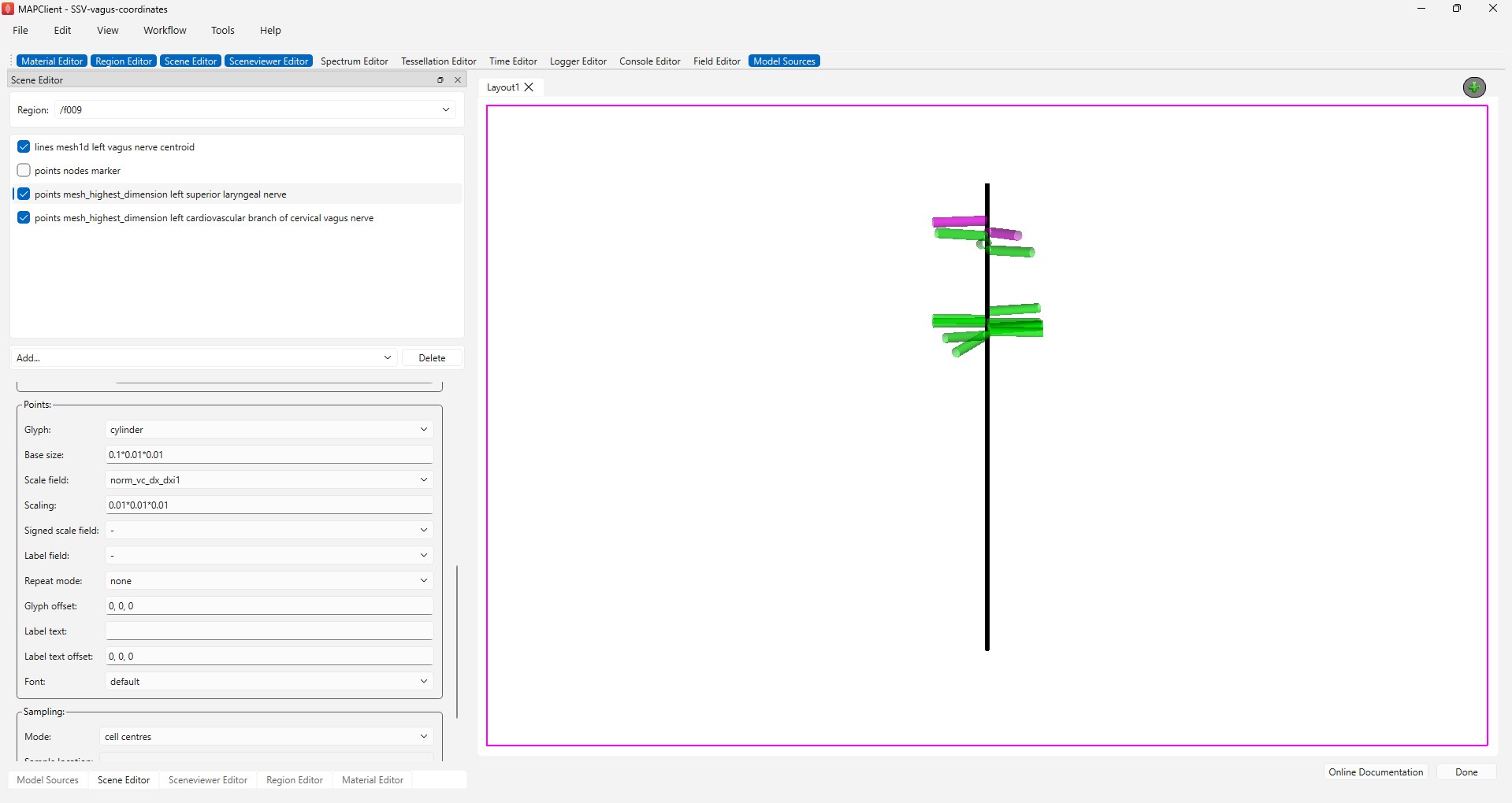
Figure 12. Visualizing the left superior laryngeal nerve in magenta50 and the left cardiovascular branch of the cervical vagus nerve in green50 for subjects f009 and f019.
Visualize branch distribution and density
Sometimes it can be helpful to visualize branches from multiple subjects on a common coordinate system without including their branch trajectories.
In the next visualization, we will generate a qualitative representation of branch density, whereby regions where multiple branches overlap appear more prominent because of the increased opacity.
Regions where branches from multiple subjects overlap can reveal areas of consistent branching, while differences in overlap can highlight inter-subject differences. This provides a qualitative view of branch density and distribution and can help identify patterns for further quantitative analysis.
First, clear the Layout view by unchecking all graphic objects in Scene Editor.
In Scene Editor, select /f009 from the Region and turn on visibility of the line graphic previously created for left vagus nerve centroid using the vagus coordinates.
Next, add element points with the following settings:
Subgroup: left superior laryngeal nerve
Coordinates: vagus coordinates
Material: magenta10
Glyph: cylinder
Base size: 0.2*0.01*0.01
Glyph offset: -0.5, 0.0, 0.0
We use magenta10 rather than magenta50 for the density plot because magenta10 is a more transparent version of the magenta material. This makes overlapping branches easier to identify and provides a better representation of branch density.
The magenta10 material can be created using the same steps described previously for creating magenta50 in the ‘Material Editor’. The only difference is to set the Alpha value to 0.1.
Next, follow the same steps to add element points for left cardiovascular branch of cervical vagus nerve from f009. Select the appropriate branch group under Subgroup and use the green10 material to visualize these branches.
Repeat these steps for any additional subjects you wish to include. In this example, repeat the process for /f019, adding graphics for the corresponding branch groups until you derive a visualization as shown in Figure 13.
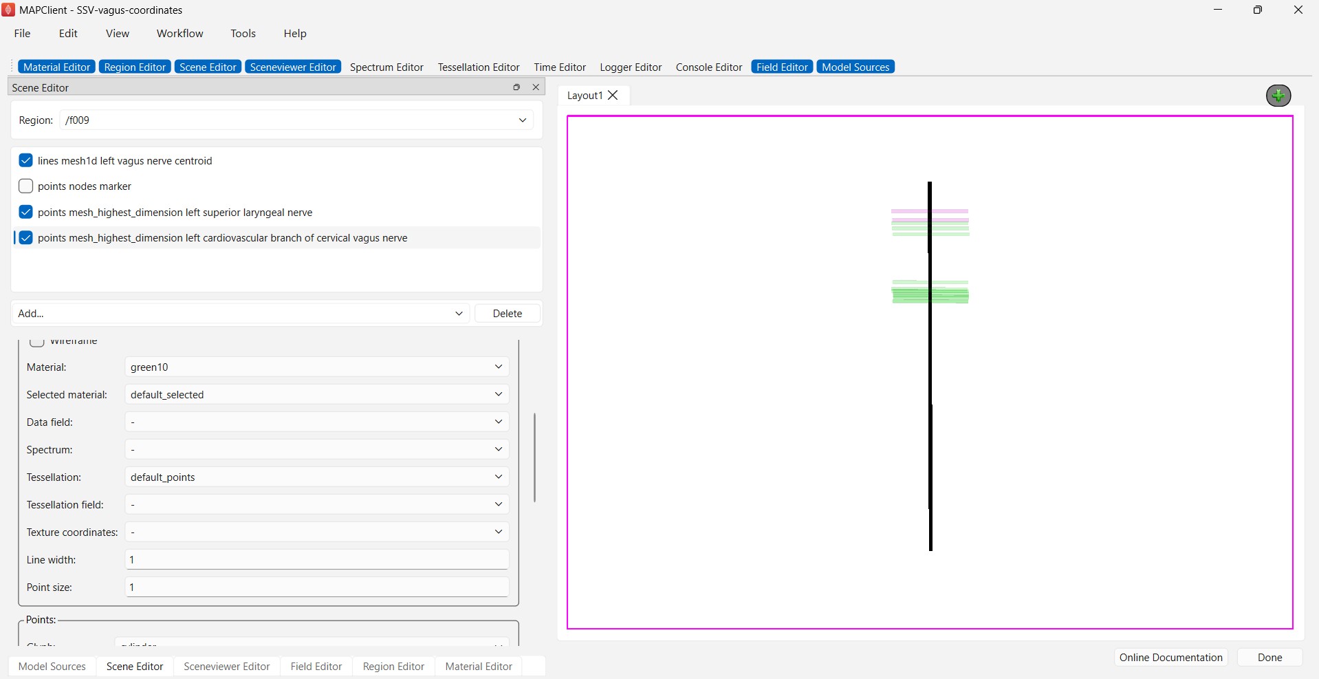
Figure 13. Distribution plot of the left superior laryngeal nerve (magenta10) and left cardiovascular branch of cervical vagus nerve (green10) for subjects f009 and f019, mapped using vagus coordinates.
Exporting the generated visualization
Once you have successfully generated the visualization required for your publication or presentation, click Done. This will end the workflow, and the visualization displayed in the Layout view will automatically be exported to the directory specified during the Argon Scene Exporter configuration step.
Summary
In this tutorial, we mapped the subject-specific scaffolds to a common coordinate framework, thereby enabling comparison of branch distributions across subjects and generation of qualitative visualizations of branch density.
Updated 2 months ago