Scaffold Mapping Tools: Mapping Image Data

In this demonstration, we are going to work through how to map segmented data onto an organ scaffold and prepare a dataset that is ready to publish on the SPARC Portal. To achieve this we are going to use the latest version of the scaffold mapping tools and a segmentation of part of the neural network from the colon of a mouse.

The latest release of the scaffold mapping tools incorporates the latest scaffolds and tools for curating SPARC datasets.

The result of this demonstration will be a SPARC dataset containing the original data, the files necessary for the visualization of the resultant scaffold map, and annotations that provide supplemental contextual information.

Table of Contents

• Setup
• Prepare Workflow
  • Step 1: Launch MAP Client Mapping Tools
  • Step 2: Configure the Workflow
  • Step 3: Execute the Workflow
• Embed the SPARC Data in a Scaffold
  • Step 1: Select a Scaffold
  • Step 2: Fitting the Scaffold with the Segmentation Data
  • Step 3: Embed the Segmentation Data into a Scaffold
• Visualize the Mapped SPARC Data on a Scaffold
  • Step 1: Adding Views
  • Step 2: Loading
  • Step 3: Mapping
  • Step 4: Visualizing

📘

Note

When the application is launched for the first time, the application may take some time to appear as it prepares its environment. When launching MAP Client, it will load the previous workflow that was used. If this is the first time MAP Client has started then the sparc-data-mapping workflow will be loaded.

📘

Note

This documentation is written for the latest version of the mapping tools. Previous versions of this documentation are available.

Older versions of this documentation:

• version 0.19.1
• version 0.17.4

Setup

First, we need to create a skeleton dataset as defined here. We will populate this dataset with files generated from the workflow. This dataset will be suitable for uploading to the SPARC Portal and sharing with others once the workflow has been successfully finished.

Second, we need to download the segmentation data to embed in the scaffold. Save this file to the primary folder of the skeleton dataset created previously.

We will take this segmentation file (in the Neuromorphological File Specification format doi.org/10.1007/s12021-021-09530-x ) as input and guide the user through the process of mapping this data into the appropriate anatomical organ scaffold. In this demonstration, we will be using a 3D digital tracing of enteric plexus in mouse proximal colon (Courtesy of Lixin Wang et al., UCLA) to describe the steps involved in mapping segmentation data to an organ scaffold.

The next three sections will take you through embedding the data in a scaffold and visualizing the embedded data.

Prepare Workflow

Step 1: Launch MAP Client Mapping Tools

Launch MAP Client Mapping Tools, found in the Start Menu under MAP-Client-mapping-tools vX.Y.Z (The X, Y, and Z will be actual numbers depending on the current stable release).

If you don't yet have the MAP Client Mapping Tools available, follow the instructions here.

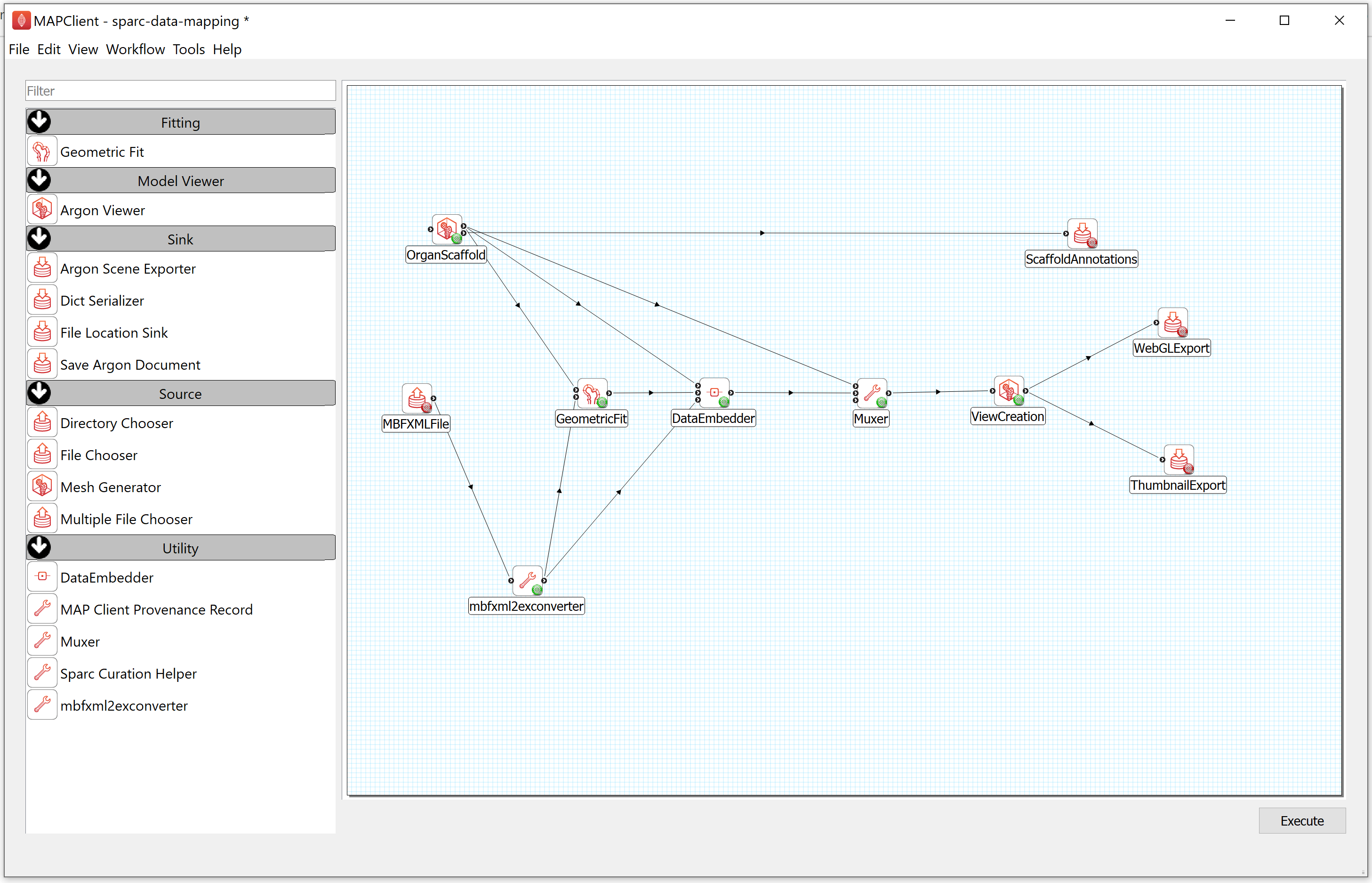
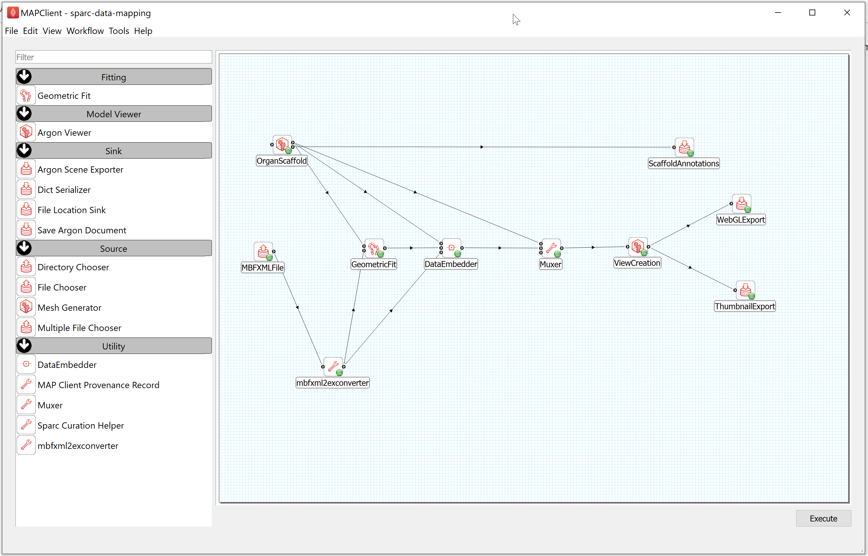
Step 2: Configure the Workflow

First, you need to prepare the workflow for execution. This means we have to configure the inputs and outputs for the workflow. The input to this task is a segmentation file in the Neuromorphological File Specification format (denoted here as MBF XML), the outputs are the DATASET_ROOT\derivative\scaffold directory in the demonstration dataset.

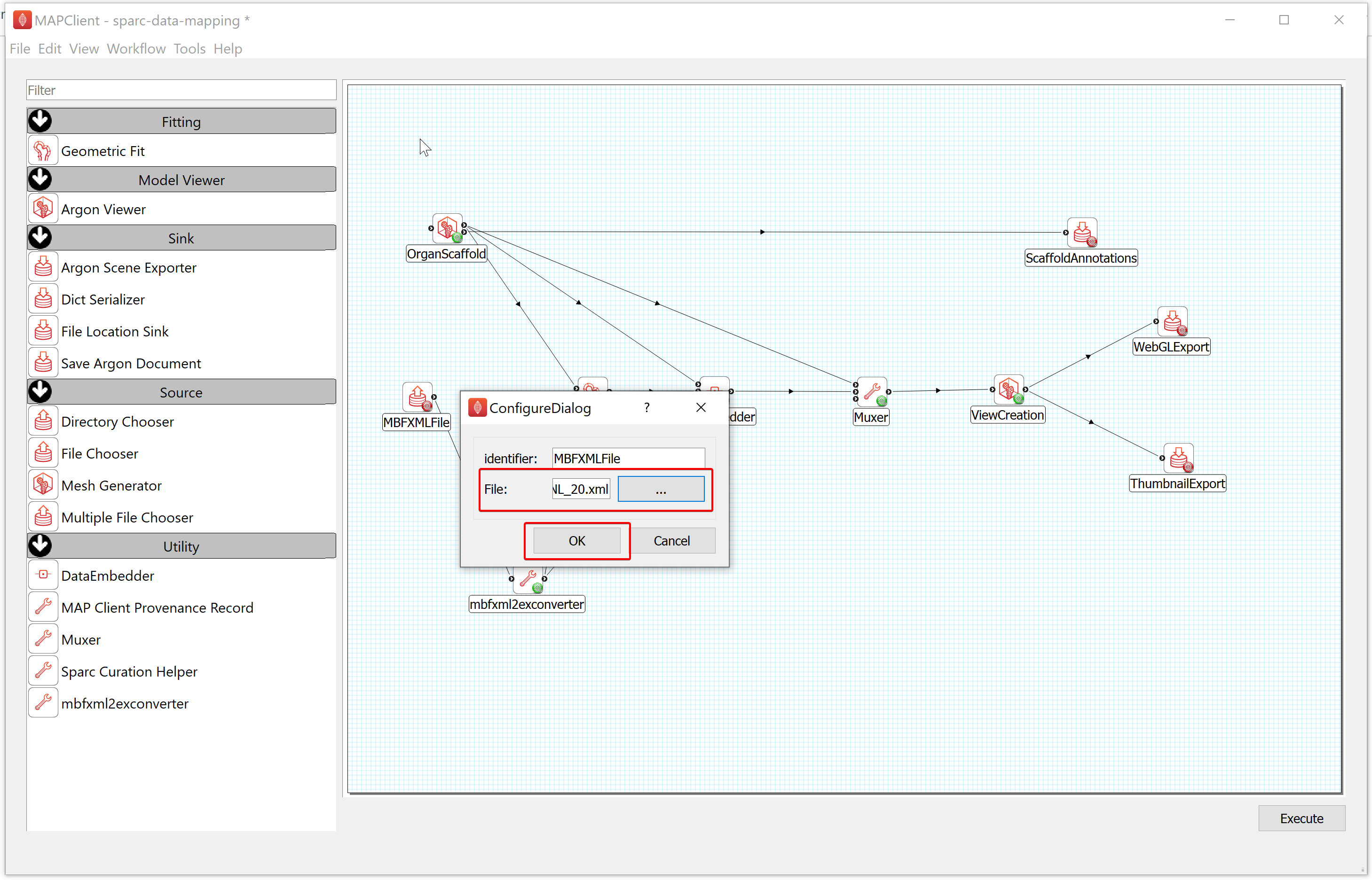
1. To configure the location of the MBF XML file providing the data to embed, follow these steps:

a) Right-click on the MBFXMLFile icon and click on the Configure option or left-click on the red gear icon to open the Configure Dialog pop-up window.

b) Using the file selection tool, select the segmentation data to embed. If you are following these instructions using the demonstration dataset then this file will be located in DATASET_ROOT\primary.

c) Click on the OK button.

📘

Note

As a result of configuring the input file for the data embedding task, the colored gear icon will change from red to green. If the colored gear icon is still red then the step is not properly configured.

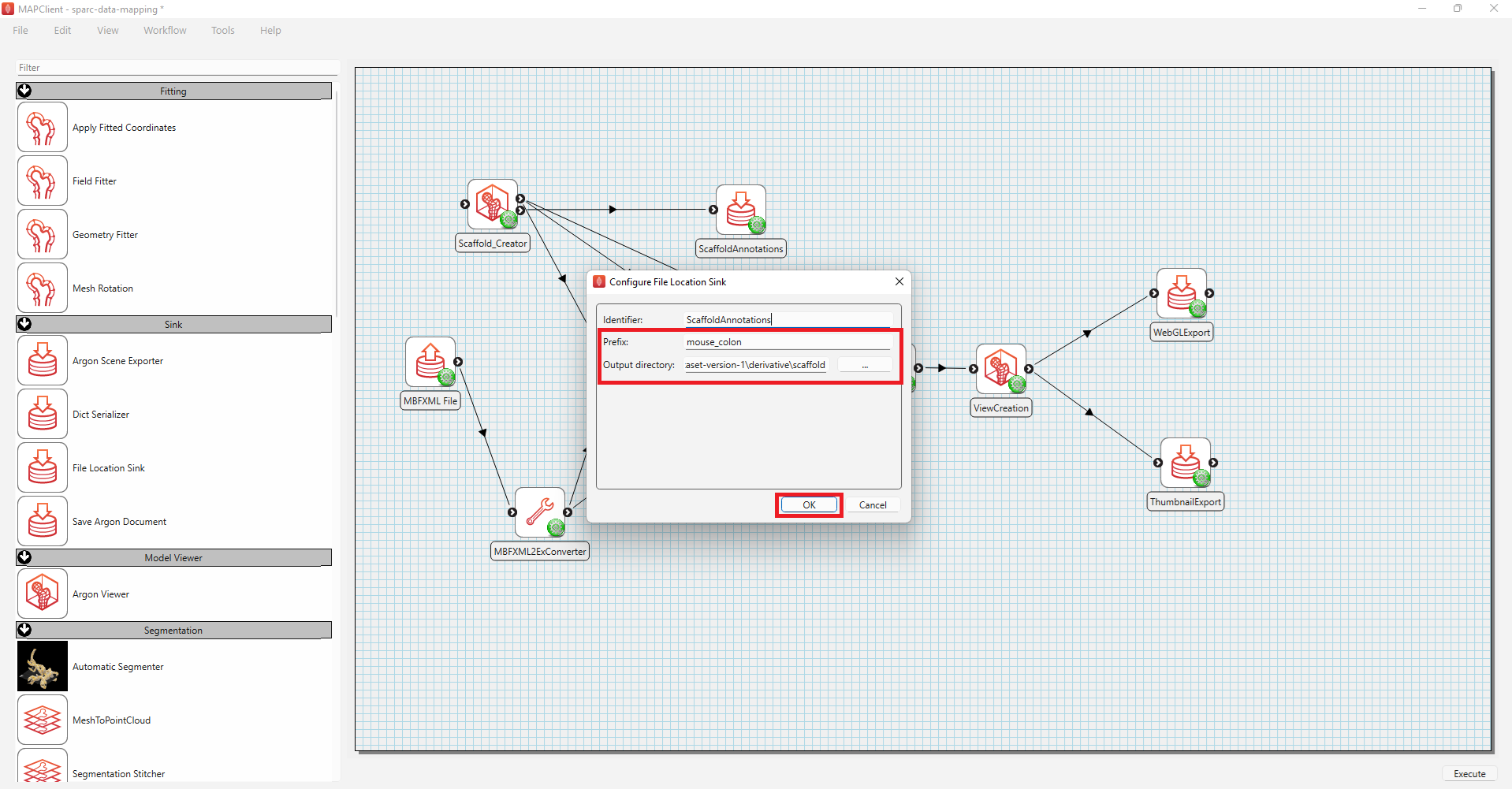
2. To configure the ScaffoldAnnotations,

a) Right-click on the ScaffoldAnnotations icon and click on the Configure option or left-click on the red gear icon to open the Configure Dialog pop-up window.

b) Select the Output directory for storing the file. If you are following these instructions using the demonstration dataset,this would be DATASET_ROOT\derivative\scaffold.

c) Click on the OK button.

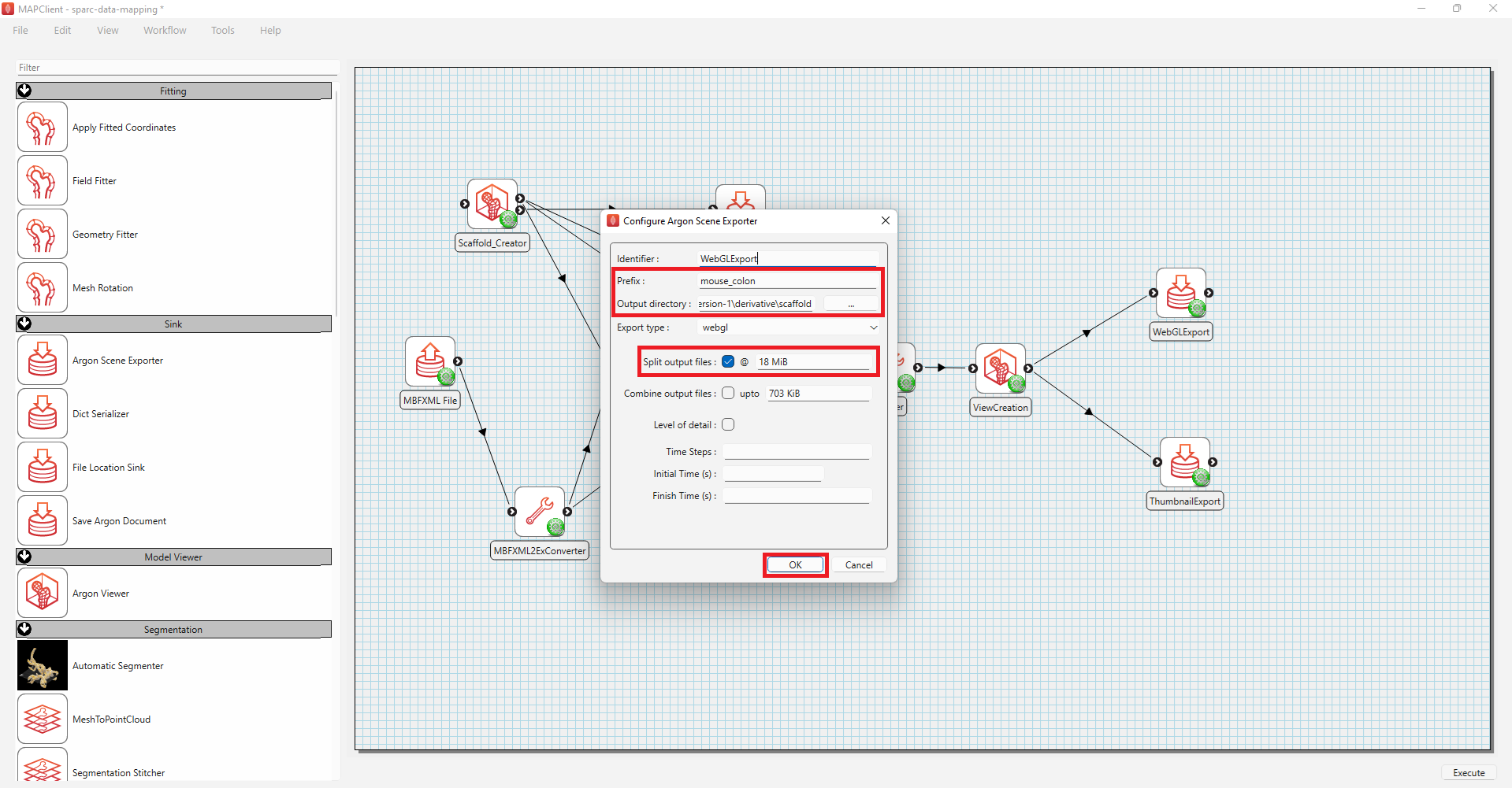
3. To configure the WebGLExport,

a) Right-click on the WebGLExport icon and click on the Configure option or left-click on the red gear icon to open the Configure Dialog pop-up window.

b) Provide a Prefix value e.g., mouse_colon.

c) Select the Output directory for storing the visualization file. If you are following these instructions using the demonstration dataset, this would be DATASET_ROOT\derivative\scaffold.

d) Click on the OK button.

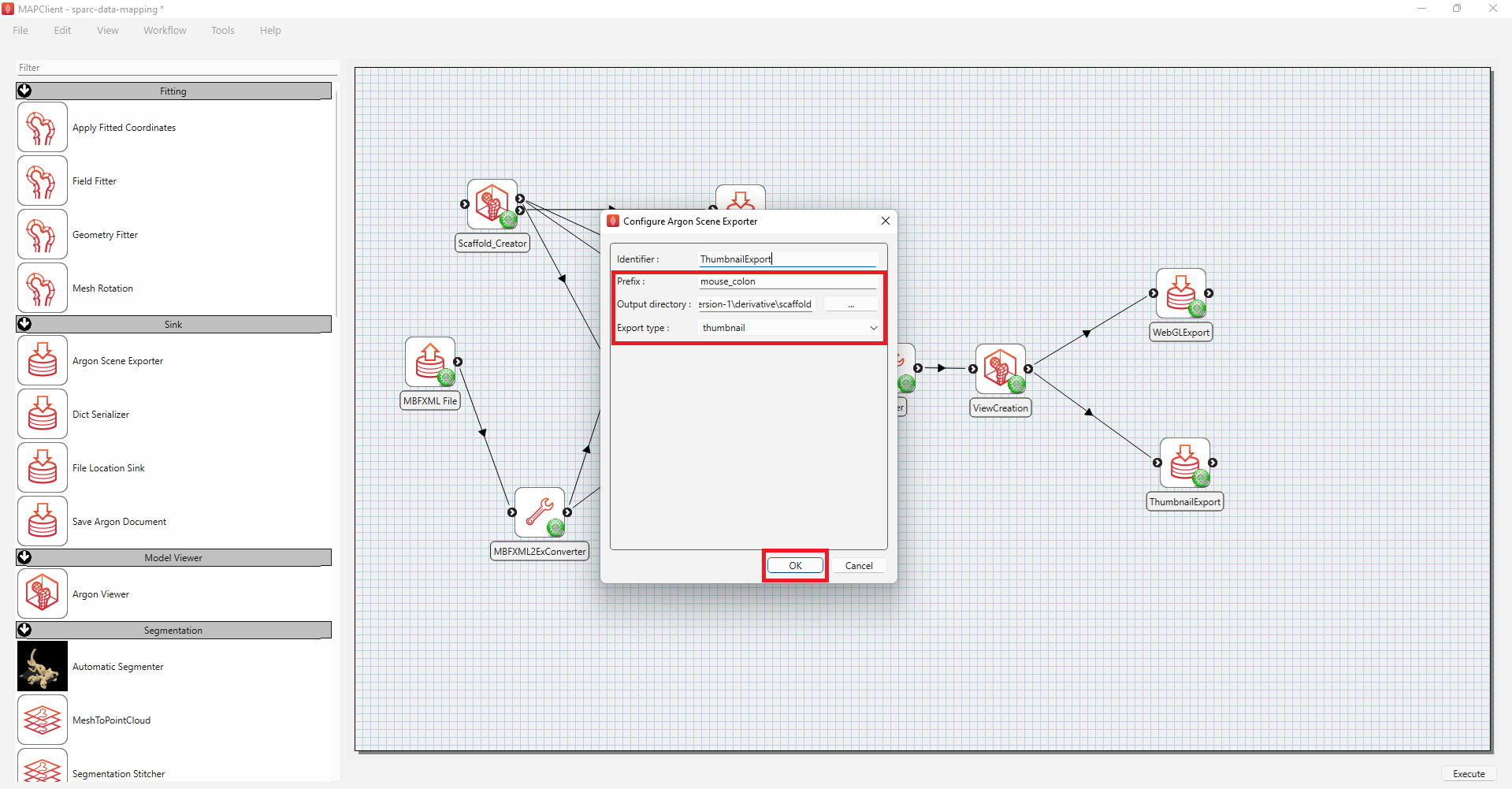
4. To configure the ThumbnailExport,

a) Right-click on the ThumbnailExport icon and click on the Configure option or left-click on the red gear icon to open the Configure Dialog pop-up window.

b) Provide a Prefix value e.g., mouse_colon.

c) Select the Output directory for storing the image thumbnail file. If you are following these instructions using the demonstration dataset, this would be DATASET_ROOT\derivative\scaffold.

d) Click on the OK button.

Next, go to the File menu (top left), then choose Save to save the workflow.

📘

Note

In the title, the asterisk (*) indicates the workflow has not yet been saved (i.e., the workflow is currently in a modified state). You are required to save it before it can be executed. To execute a workflow, the workflow must not be in a modified state and all steps must be successfully configured. A successfully configured step shows a green gear icon.

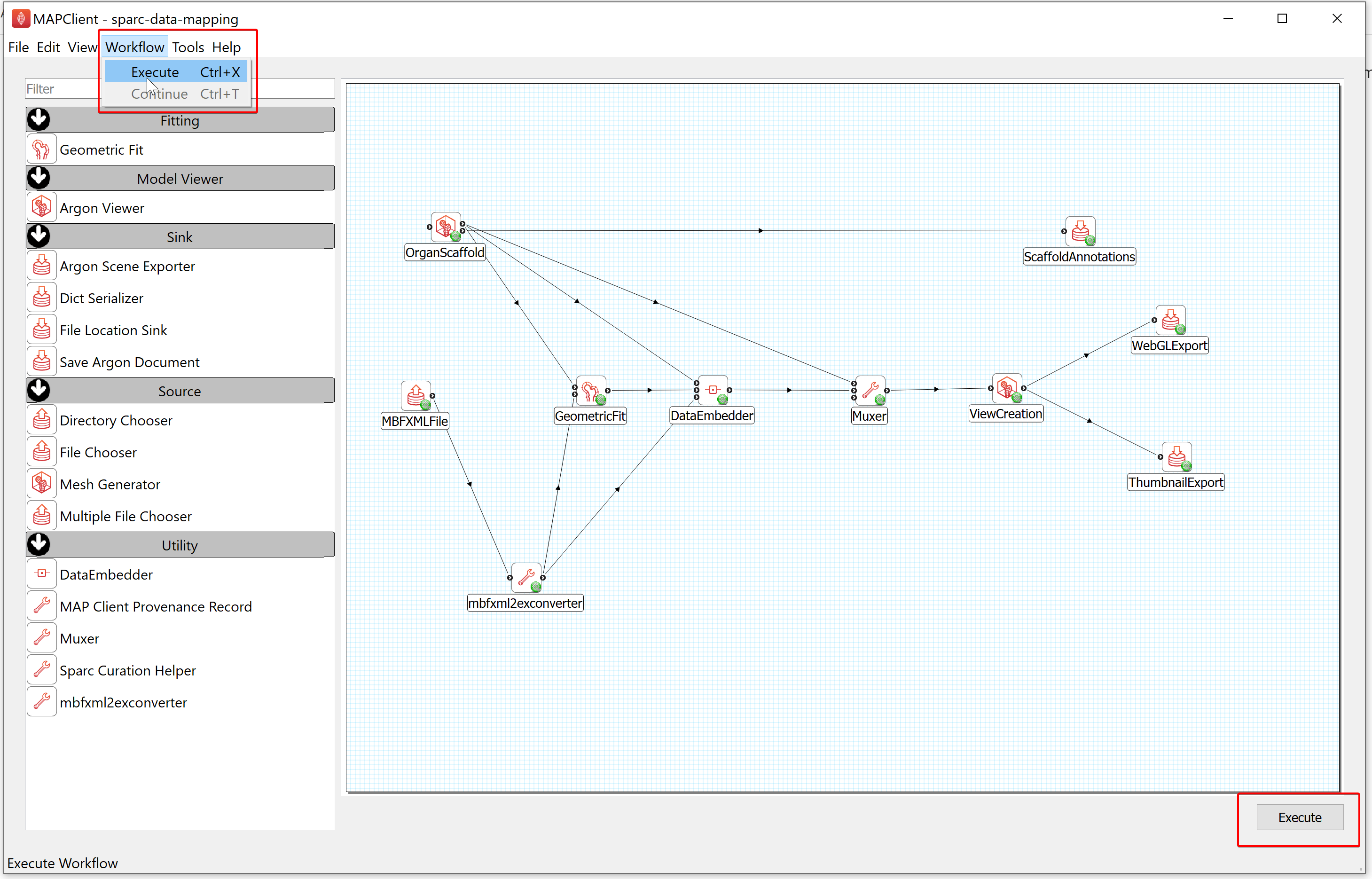
Step 3: Execute the Workflow

After configuring the workflow, you can run this workflow by selecting the Execute item in the workflow menu or clicking on the Execute button located at the bottom right of the window.

Embed the SPARC Data in a Scaffold

Step 1: Select a Scaffold

The scaffold creator step allows us to select a scaffold from a predefined list of scaffolds and generate a representation of it. We can change parameters in the interface to alter the geometric representation of the scaffold. For organ scaffolds, like the colon, we also have predefined parameter sets for different species, e.g., mouse. By selecting an organ scaffold and then choosing a species for that scaffold we can generate a scaffold onto which we can map data to.

For our demonstration dataset we need to generate a mouse colon scaffold to map the segmentation data to. We can do this with the following instructions:

In the Mesh type drop-down list, choose the organ you need to fit. For the demonstration dataset we will choose the 3D Colon 1 mesh type.

Following this, select the species of interest (for the demonstration dataset choose Mouse 1) under the Parameter set dropdown menu. Click on the View All button.

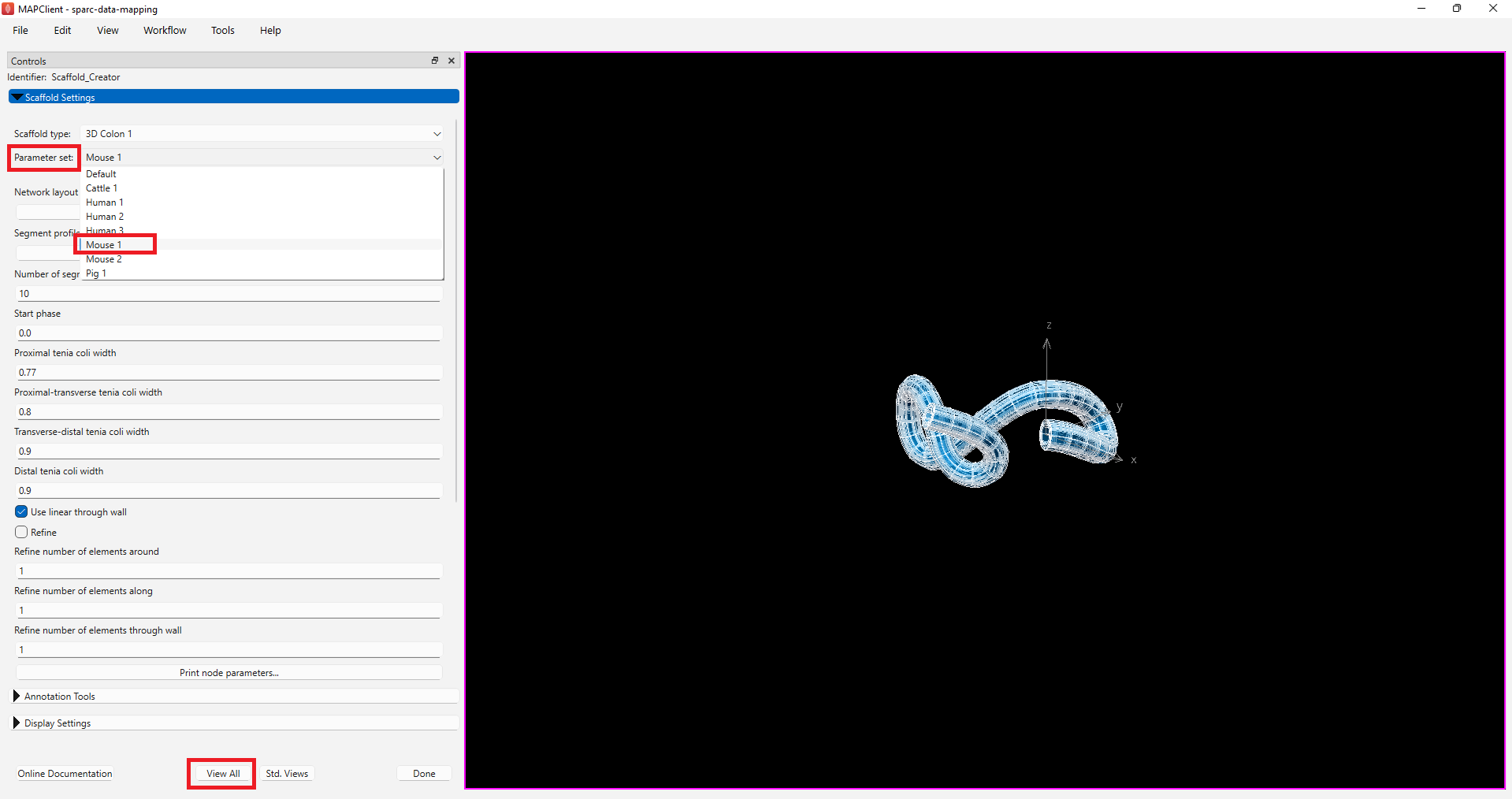
When you have chosen the mesh that you are fitting the data to, click on the Done button.

Step 2: Fitting the Scaffold with the Segmentation Data

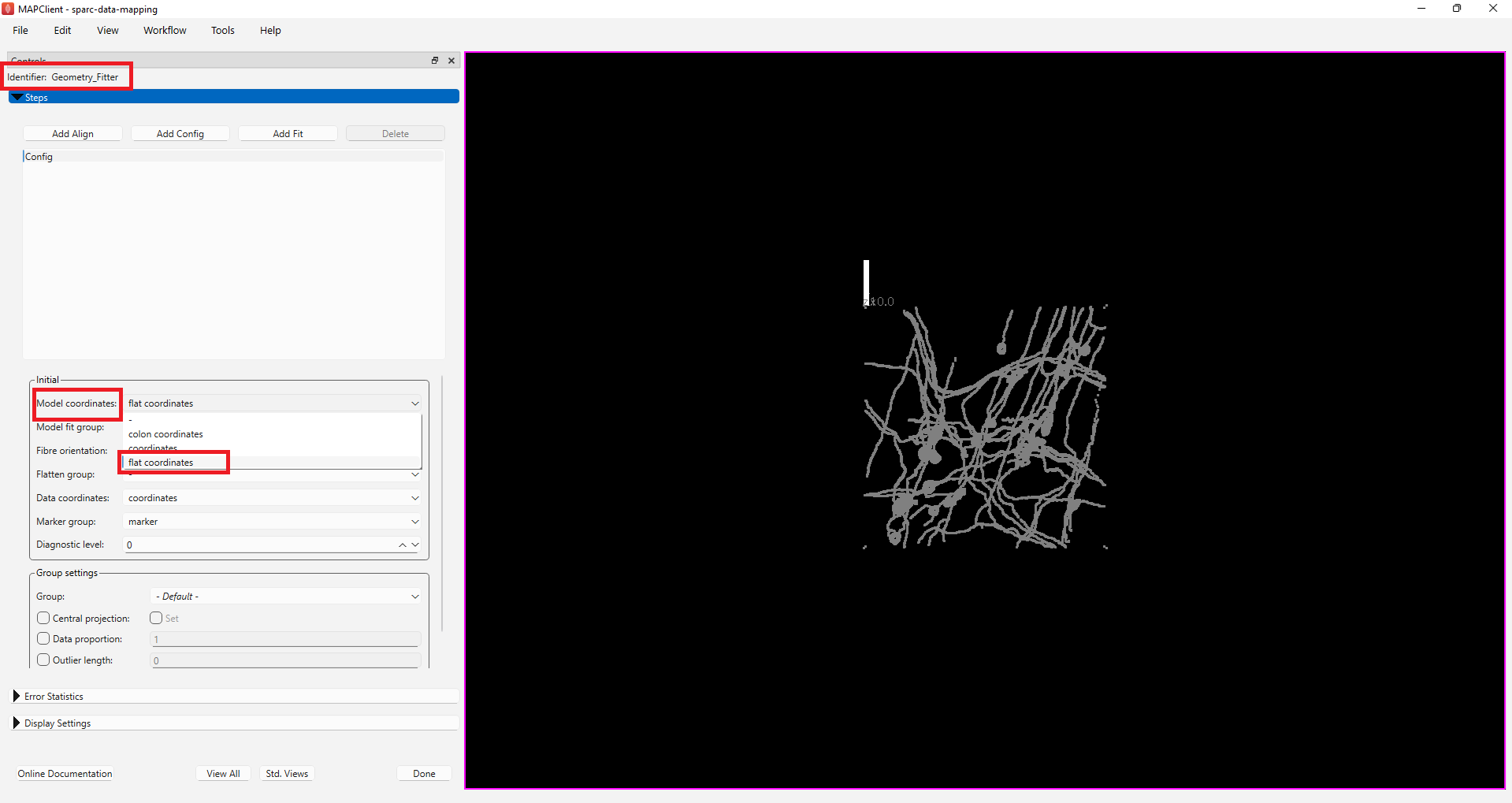
For the demonstration dataset the scaffold model and data are in different coordinate systems. In our demonstration we can change the coordinates the model is displayed in to flat coordinates, thus bringing the scaffold model and data into the same coordinate system (albeit on different scales). To do this, select flat coordinates from the Model coordinates chooser.

Now, to align the data to the model we construct a fitting pipeline. The fitting pipeline is created by adding: alignment, config, or fit steps. For the demonstration dataset the fitting required is a simple rigid body transformation. The way we choose to construct the fitting pipeline is a matter of personal choice.

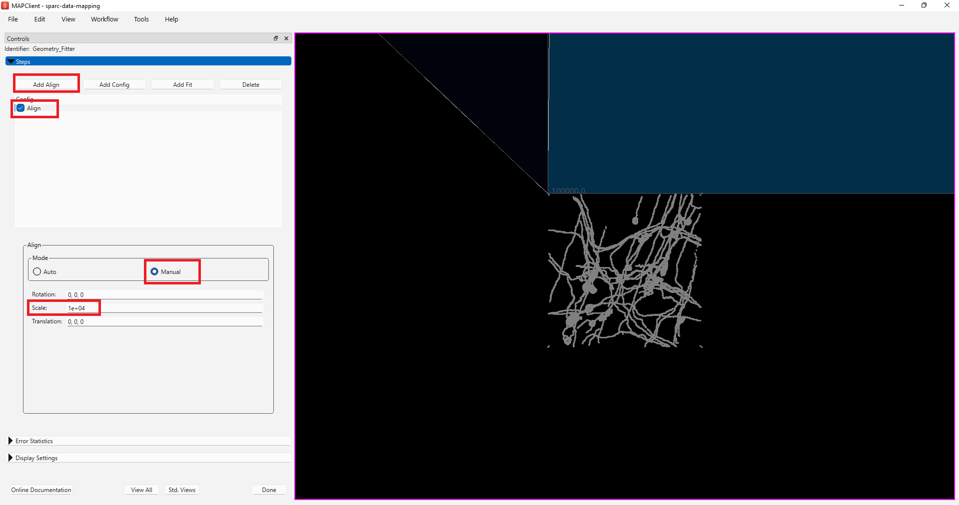
For the demonstration dataset, we will create two steps. The first will scale the model to the correct size and the second will position the model over the data correctly. To do this, click on the Add Align button. Enter a Scale value of 10000 to bring the scaffold to the same scale as the data, the example data is provided in micrometers while the scaffold is in millimeters. Hence, you will enter 10000 under Scale to bring the scaffold to the same scale as the data. The step action is not affected until the checkbox in front of the step is checked. This allows us to control when the fitting is performed, which is useful when a significant amount of processing is required to perform the fit step. When we check the Align box the fit action is performed and the outcome is rendered in the scene.

For the demonstration dataset, the next step is to move the data to the correct location on the scaffold, we can do this using the information of where the data was extracted from the organ. Here the sample was obtained 2mm from the mesentery margin, about 2cm from the start of the proximal colon, and was derived from the interface between the circular and longitudinal muscle of the colon.

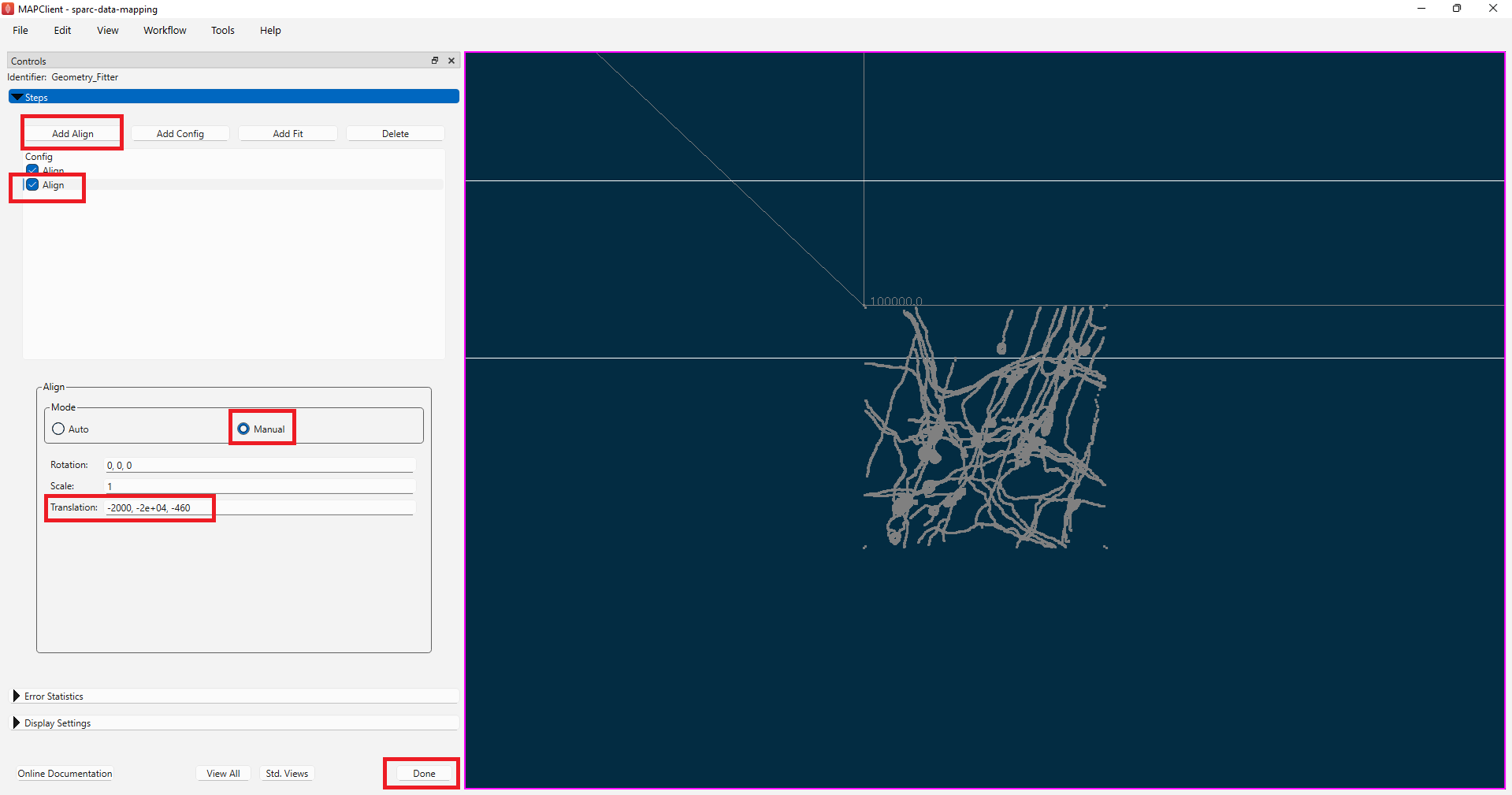
To finish registering the demonstration data to the correct location, add another Align step by clicking on the Add Align button. In this case, the correct value for the translation is [-2000, -20000, -460].

When you have finished aligning the scaffold model to the data, click on the Done button.

📘

Note

In cases where the data of the 3D volume or surface contours of the organ is available to get the scaffold close to the shape of the organ at the time of data collection (for example, intrinsic cardiac nervous system image of rat hearts, microCT images of rat stomach vasculature), steps additional to the alignment step will be needed to fit the scaffold to the segmentation contours. The steps required for such geometric fitting are described here in detail. If you need help with geometric fitting of your data, please contact MAP-Core or join us during our monthly MAP-Core’s Open Office Hour.

Step 3: Embed the Segmentation Data into a Scaffold

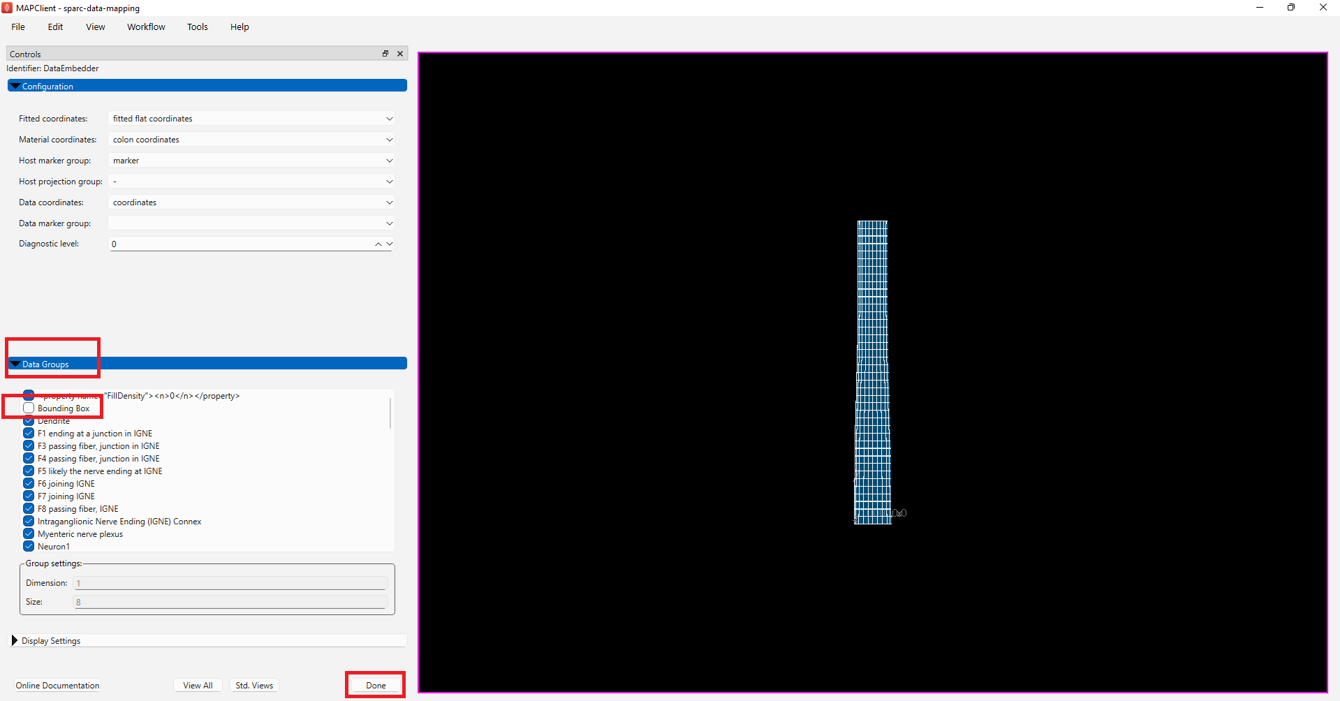
For this step, the configurations like Fitted coordinates, Material coordinates, and Data coordinates are auto-generated. We will uncheck the Bounding Box option under the Data groups as the bounding box was used for alignment and does not need to be embedded on the scaffold.

Visualize the Mapped SPARC Data on a Scaffold

To visualize the data we use the Argon Viewer step. The Argon Viewer step is a general visualization creation and management tool. Where we pass in source files, obtained from the output of previous steps, which we can use to read data from and construct a visualization for. The output of this step is an Argon document that completely describes our visualization.

Step 1: Adding Views

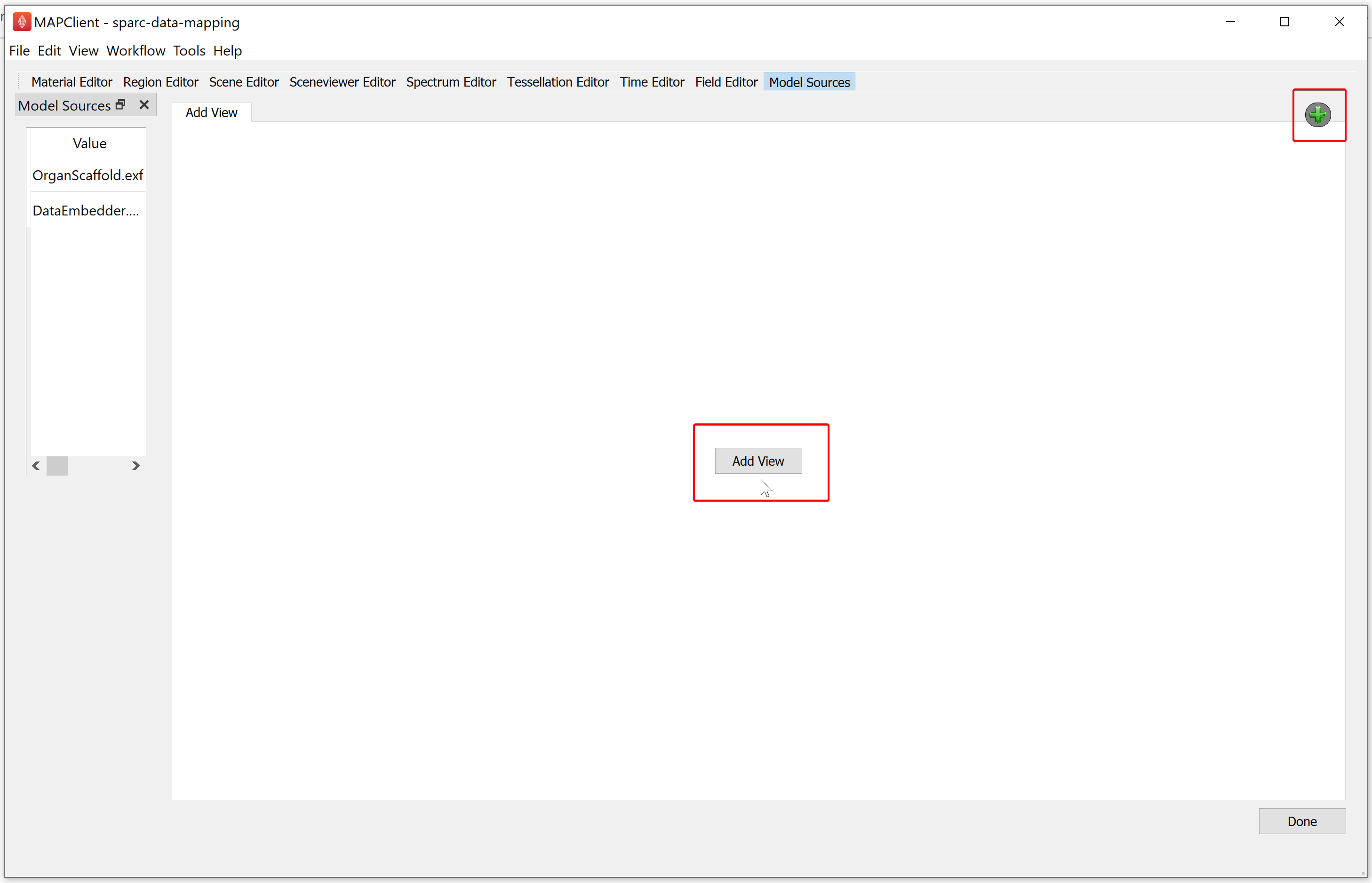
The first task we need to perform is adding a view. A view is a window that shows a visualization from a particular viewpoint. Initially we have no views, to add a view we click either the Add View button on the main widget or the green plus icon in the top right corner of the main widget. Once we have added our first view only the green plus icon will be available to add further views.

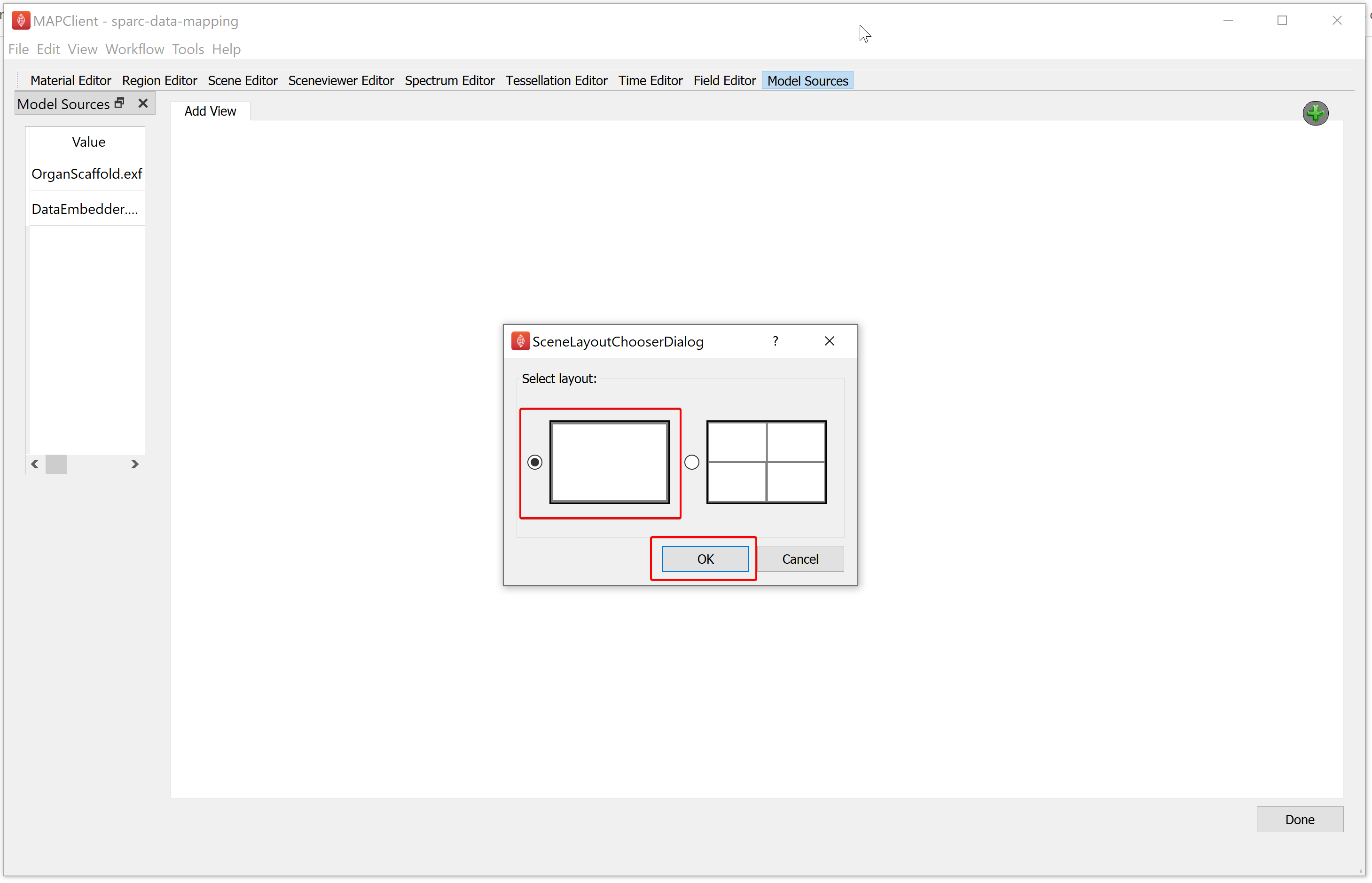
Clicking on either the Add View button of the green plus icon will show the Scene Layout Chooser window. Select the single view layout from the Scene Layout Chooser window, as only this layout is suitable for generating files for web visualization. At this time, we do not support exporting the four view layout into a web visualization.

Similarly, add another single view layout as explained above. We can rename a view by double-clicking on the tab header. For the demonstration dataset, we will rename the first layout as default, followed by renaming the second layout as proximal.

📘

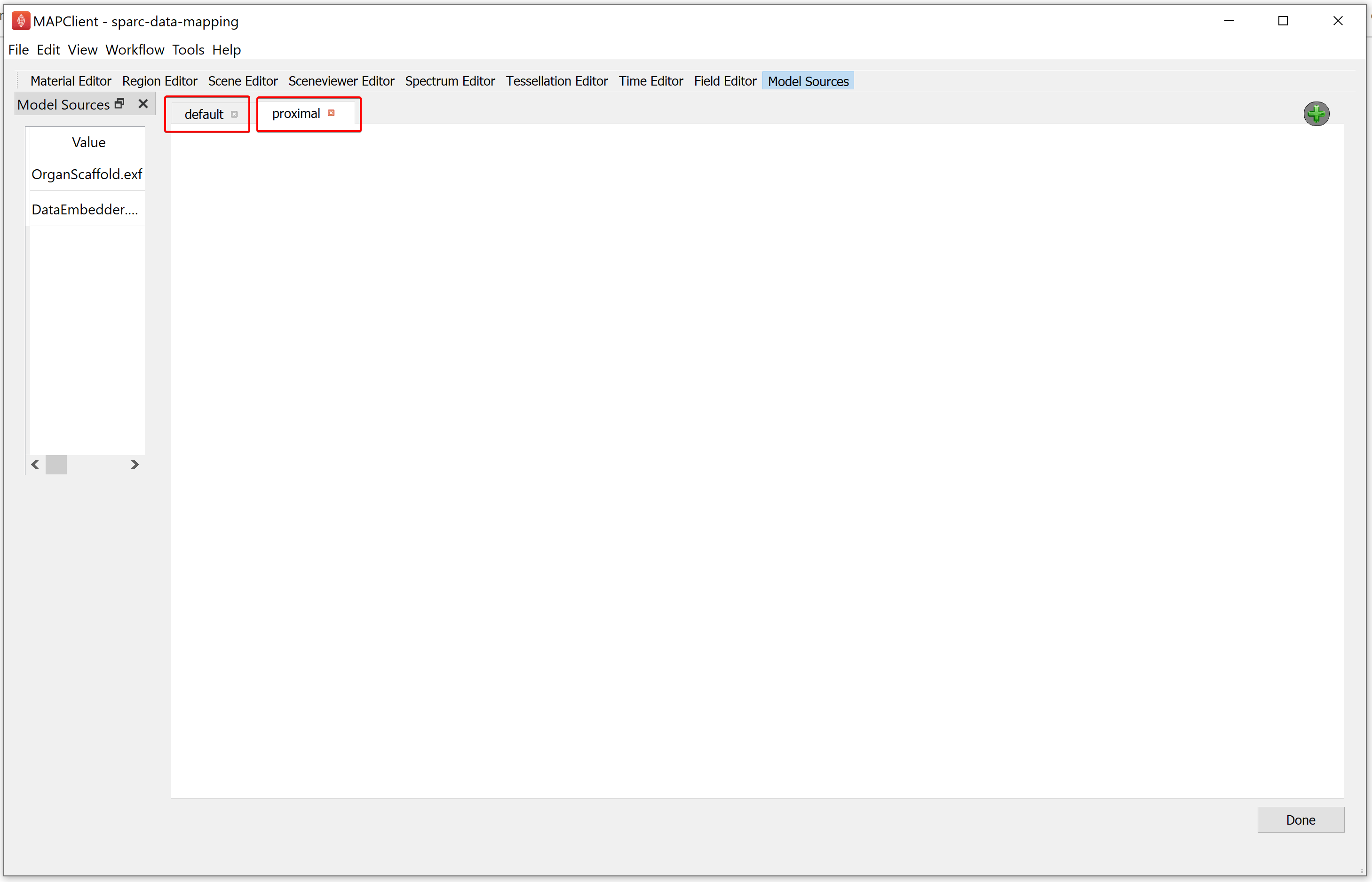
Note

It is better to use unique names for each view.

Step 2: Loading

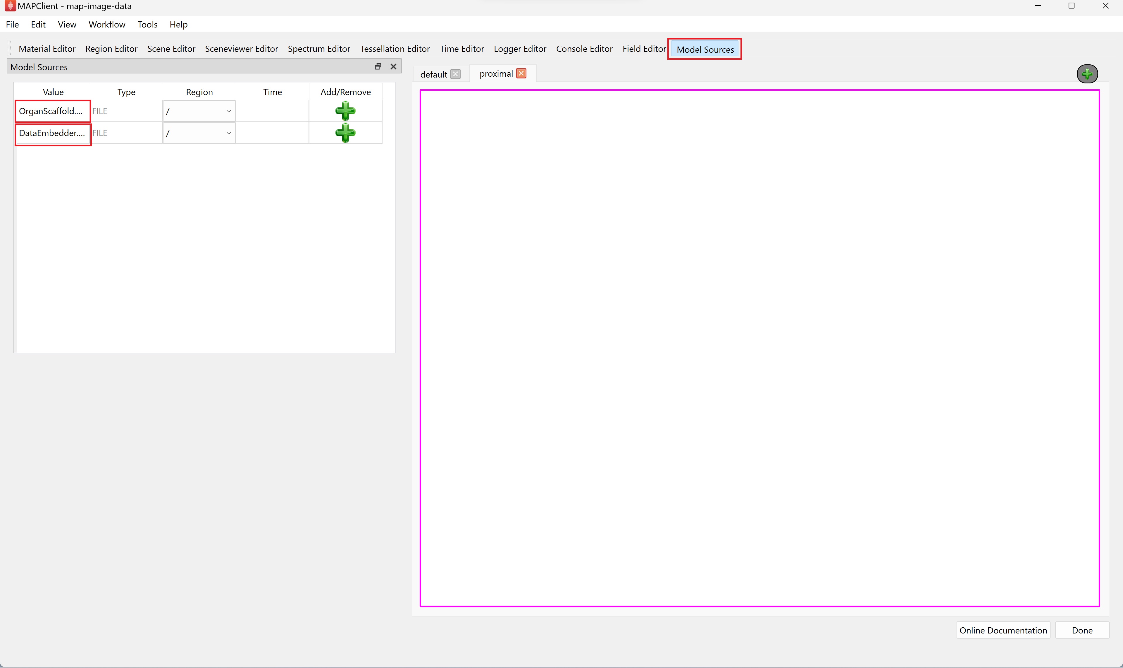
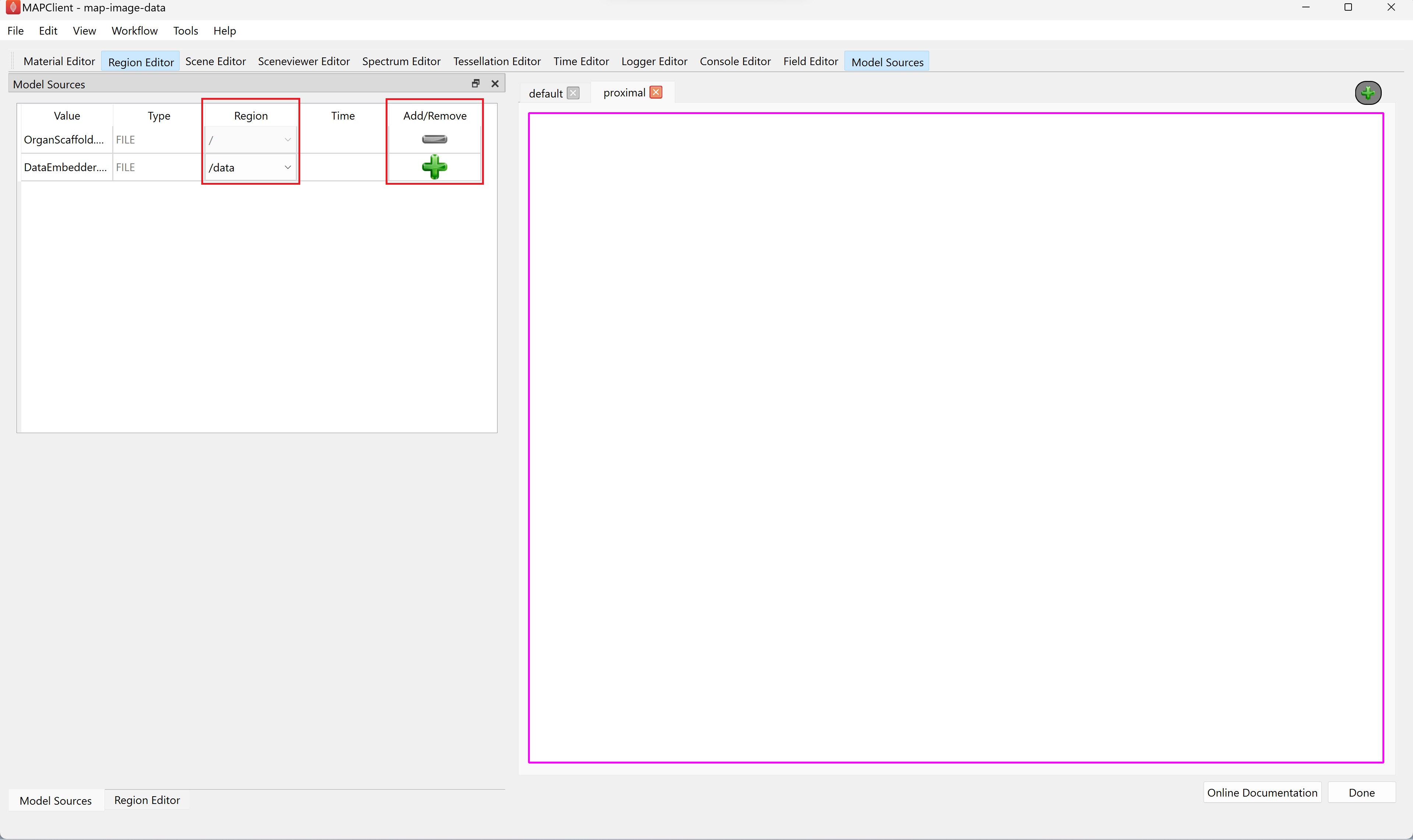
The Model Sources editor allows you to add the resources from a file into the visualization of the scaffold map. This editor lists all the available resources that have been provided to the step. For the demonstration dataset these are the organ scaffold and the embedded data files.

You must load a file into a region, if the Add/Remove column contains a green-colored plus icon this indicates that a region has not been assigned for the corresponding file resource.

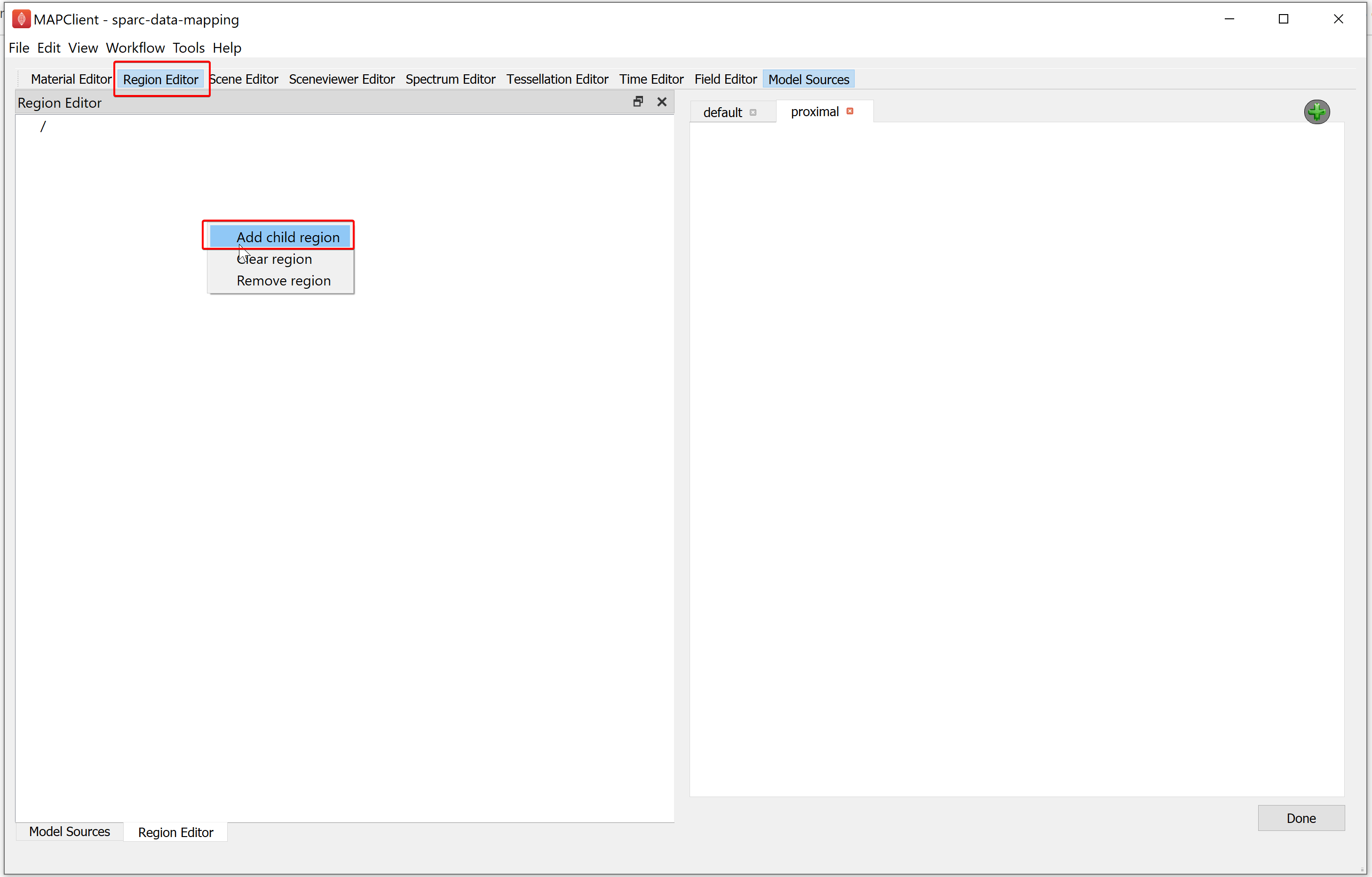
To manage regions, we use the Region Editor. While we can load multiple files into the same region this is not good practice and is heavily discouraged. We create new regions by right-clicking on the parent region of the new region. From the popup menu select the add child region entry. We can rename a region by double-clicking on the region and entering an alpha-numeric value. For the demonstration dataset we will create a child region and name it data.

Use the Model Sources editor to load a file into a region. To assign a region to load a file into, first click inside the Region column cell and a Field chooser will appear from which you can choose an existing region.

When a region has been assigned to a field resource the Add icon changes from grey to green to signify that it is now enabled. If you click on the green-colored plus (Add) icon the file resource will be loaded into the assigned region. The grey-colored minus (Remove) icon signifies that we have applied the file to the assigned region.

For the demonstration dataset we want to load the organ scaffold into the root region (/) and the embedded data into the data region (/data). Use the Model Sources editor to do this by assigning the appropriate region to each file resource and clicking the green-colored plus (Add) (for both file sources).

📘

Note

The grey-colored minus (Remove) icon to remove a file from the assigned region is currently disabled. Removing an assigned file from a region will be available in a later release of the software.

Step 3: Mapping

To map the embedded data to the model we need to create an embedded field which maps our embedded data into the model. We do this by setting up a field pipeline. We shall show how this is done using the demonstration dataset.

With the demonstration dataset, we will need to create four fields in the Field Editor to embed the segmentation data into the scaffold.

The first field we will create is an argument field, this field accepts another field as an argument and creates a placeholder for it. This is very similar to an argument for a function.
The second field we will create is a find mesh location field, this field will look up the location of the values given through the argument field in the current mesh.
The third field we will create is an embedded field, this field will give the value of the source field evaluated at the found mesh location.
The fourth field we will create is an apply field, this field will bind a field to the argument field allowing its values to be returned as the values calculated from the target field.

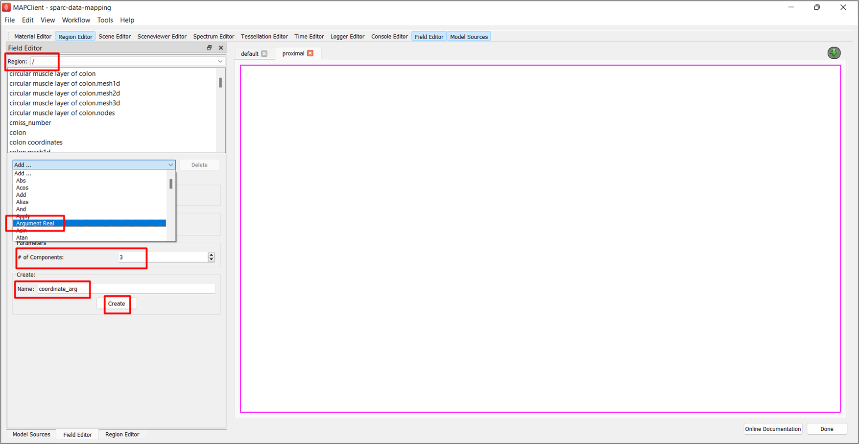
For creating the first field, go to the Field Editor,

1. Select the root (/) region from the Region chooser.

2. Click on Add ..., select the Argument Real field type.

3. Set the # of Components for the field value to 3.

4. Enter the Name as coordinate_arg.

5. Click the Create button.

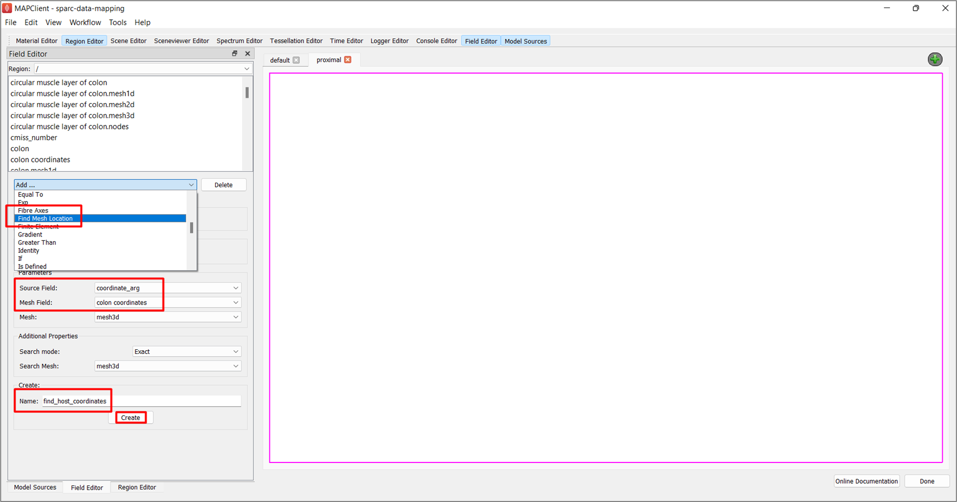
To create the second field, in the Field Editor window,

1. Click on Add ... button, select the Find Mesh Location field type.

2. Set the Source Field chooser value to coordinate_arg.

3. Set the Mesh Field chooser value to colon coordinates.

4. Enter the Name as find_host_coordinates.

5. Click the Create button.

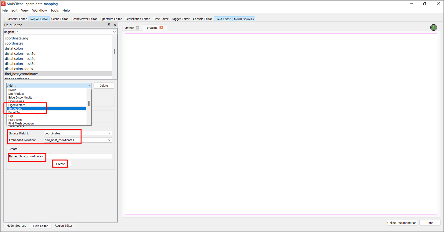
To create the third field, in the Field Editor window,

1. Click on Add ..., select the Embedded field type.

2. Set the Source Field 1 chooser value to coordinates.

3. Set the Embedded Location field to find_host_coordinates.

4. Enter the Name as host_coordinates.

5. Click the Create button.

The creation of the fourth field is slightly different from the previous three.

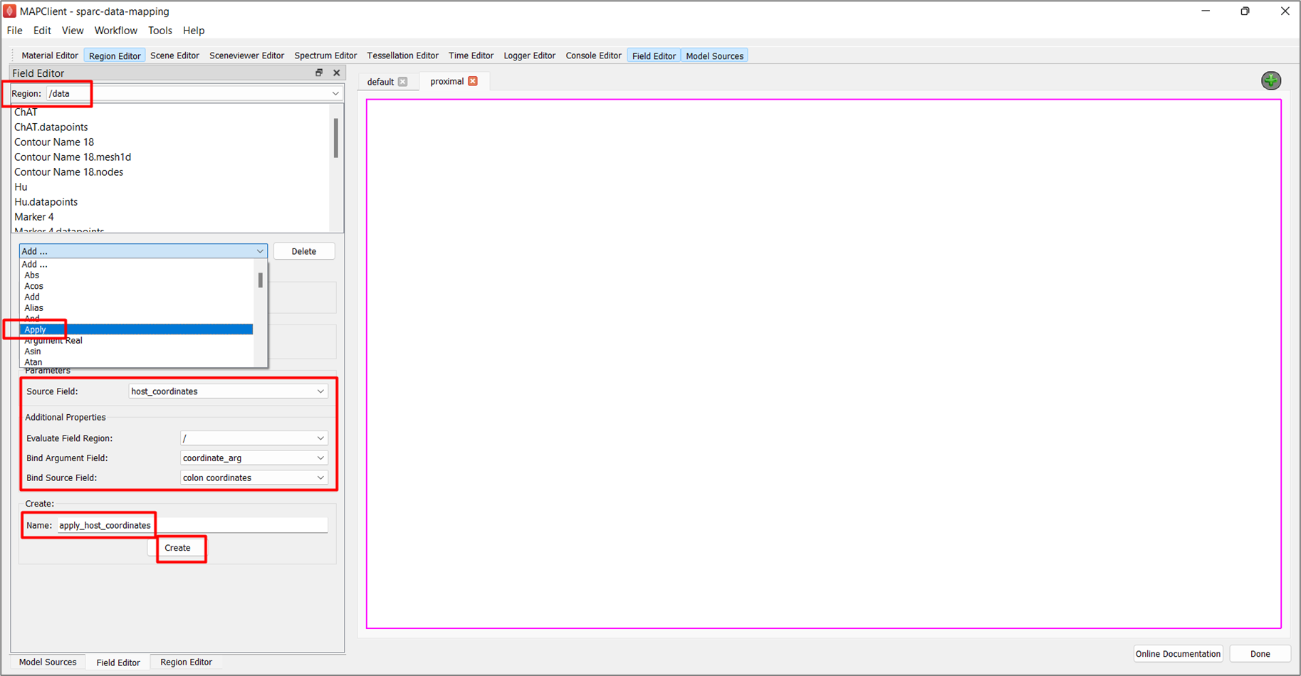
To create the fourth field, in the Field Editor window:

1. Select the /data region from the Region chooser.

2. Click Add ... option, select the Apply field type.

3. Set the Evaluate Field Region as root ( / ).

4. Set the Source Field to host_coordinates.

5. Set the Bind Argument Field to coordinate_arg.

6. Set the Bind Source Field to colon_coordinates.

7. Enter the Name as apply_host_coordinates.

8. Click the Create button.

With these four fields created we have defined a field pipeline that will look up locations in the host mesh and evaluate the bound field at this location. To see the embedded data at its embedded location we apply the mapped host coordinates to the graphics visualizing the embedded data. We do this through the Scene Editor.

Step 4: Visualizing

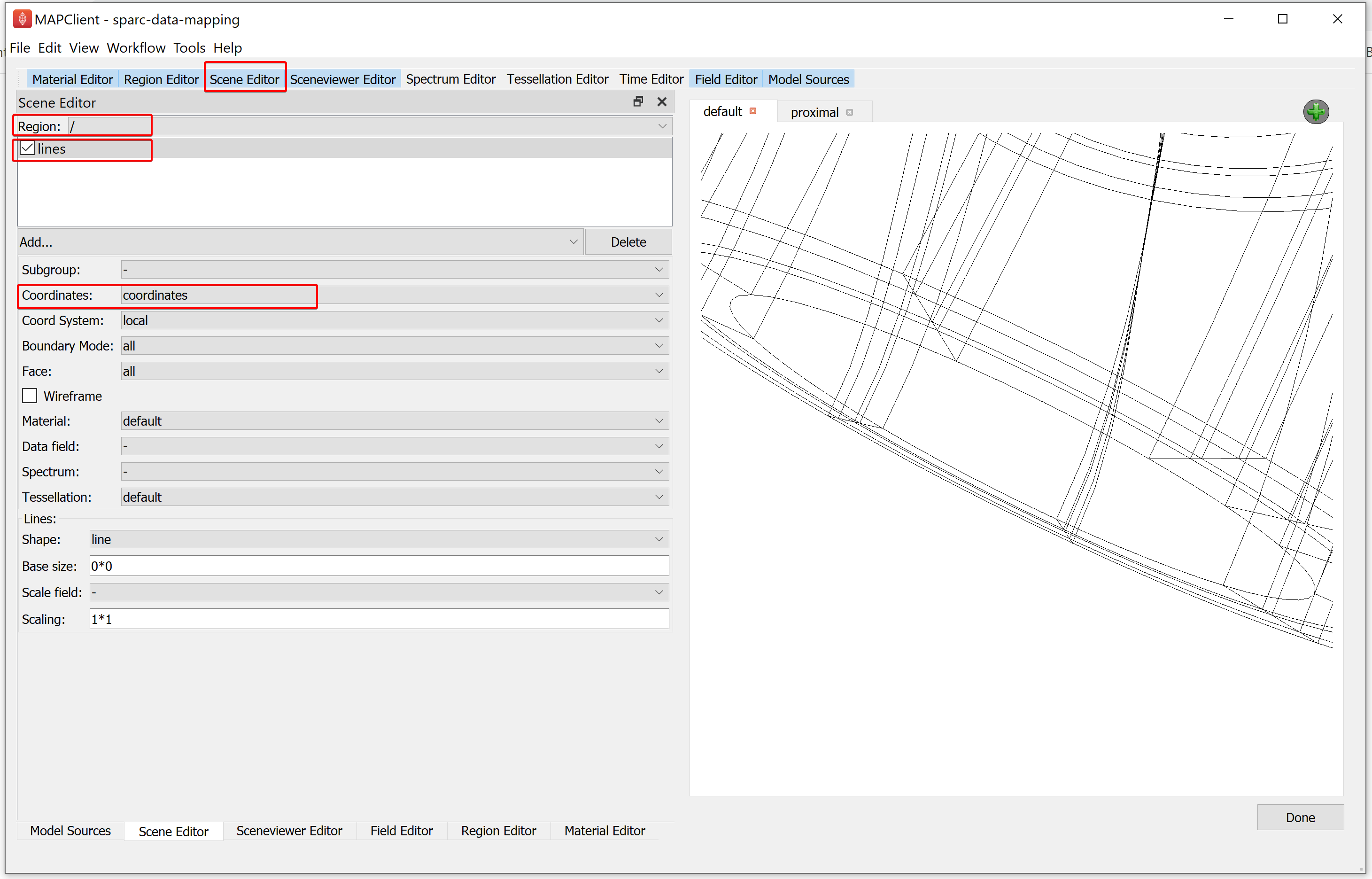
To visualise the scaffold and data we must add graphical elements that combine to create a picture of our scene. To do this, go to the Scene Editor, select the Region as / and select lines from the add graphics chooser. From the options for lines, set the Coordinates field value as coordinates.

When working with computer graphics it is important to know that we have a very limited viewing frustum to work with. Now that we have added something to look at -- lines -- we need to make sure that we are actually looking at them. It is very likely that we will not be looking at the lines we have just added. To bring our view to bear on the lines we added, we use the Sceneviewer Editor and the View All button to reset the view to look at all visible objects in our scene. Before we use the View All button we must select the view to view all of. When we click on a view we will enable the Sceneviewer Editor to read and modify that view, we can see that a view is enabled and accessible through the Sceneviewer Editor because a purple outline appears around the active view.

Next, select the default view (selected view is indicated by a purple outline) and go to the Sceneviewer Editor and click on the View All button to view scaffold.

We can set the visualization to only show the boundary surfaces in the Scene Editor. Select the lines in the graphics listing. From the lines options set the Boundary Mode to boundary and Face value to xi3 = 1. For 3D models we should perform this action for all graphics, if it makes sense for the visualization we are trying to achieve. When the final output is destined for a webpage, as it is here, the less graphics we have the better. We should therefore look to create our visualization with the least amount of graphics as possible. Webpages don't have as much graphical rendering power as a desktop application does, and a webpage is also comparatively very slow to render large graphical elements.

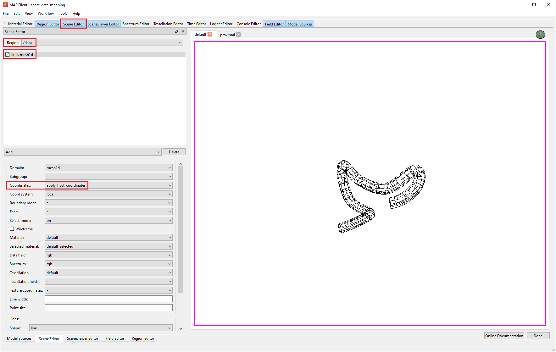
Go to the Scene Editor, select the Region as /data and select the lines in the graphics listing. From the options for lines, set the Coordinates field value as apply_host_coordinates. Next, go to the Sceneviewer Editor and click on the View All button to reset the view.

Go to the proximal view tab and make the view active. Use the Screenviewer Editor and View All button to view everything we have made visible with our line graphics.

Now we modify the proximal view to show the proximal section of the mouse colon and the embedded segmented data. We can use the computer mouse to move the scene around, and with zoom, get a close-up look of where the segmented data lies on the mouse colon.

Alternatively, we can use the scene editor to temporarily hide the lines for the colon and use the View All button in the sceneviewer editor to automatically bring the embedded segmented data into view. To do this, for the Region in the scene editor choose / and uncheck the check box next to the lines entry.

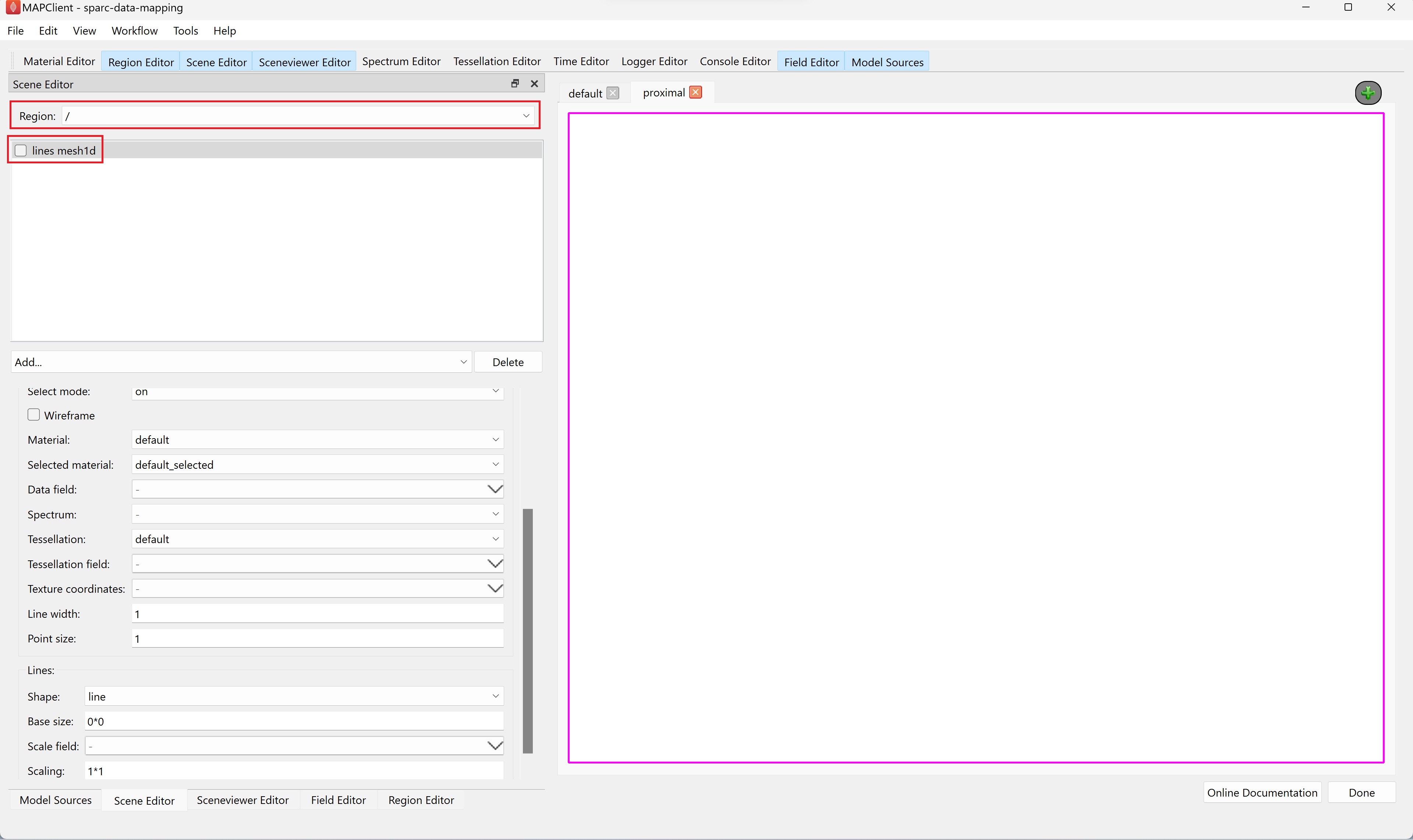
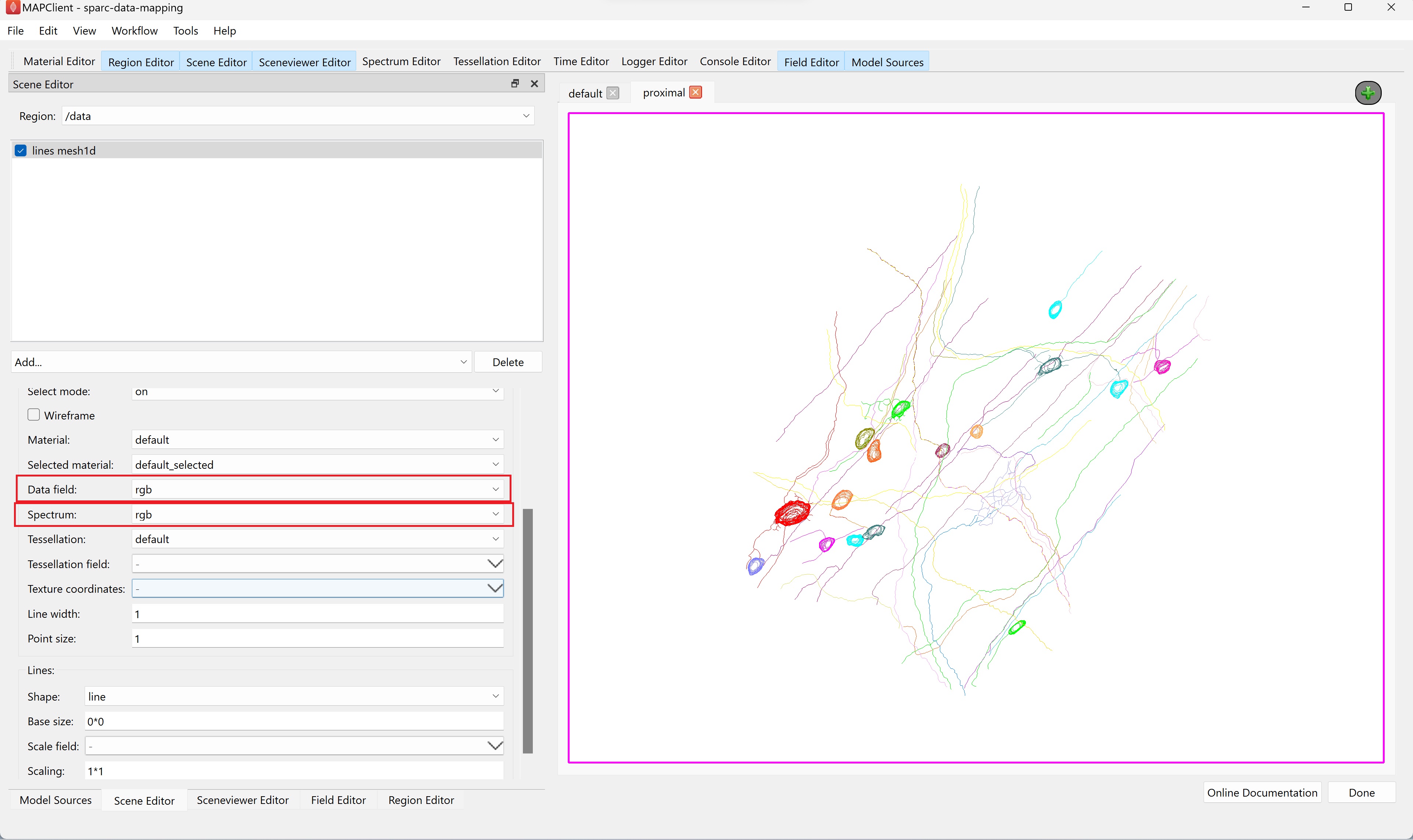
After clicking the View All button in the sceneviewer editor we can see the embedded segmented data.

Set the Data field and Spectrum parameters of the lines in the /data region to rgb.

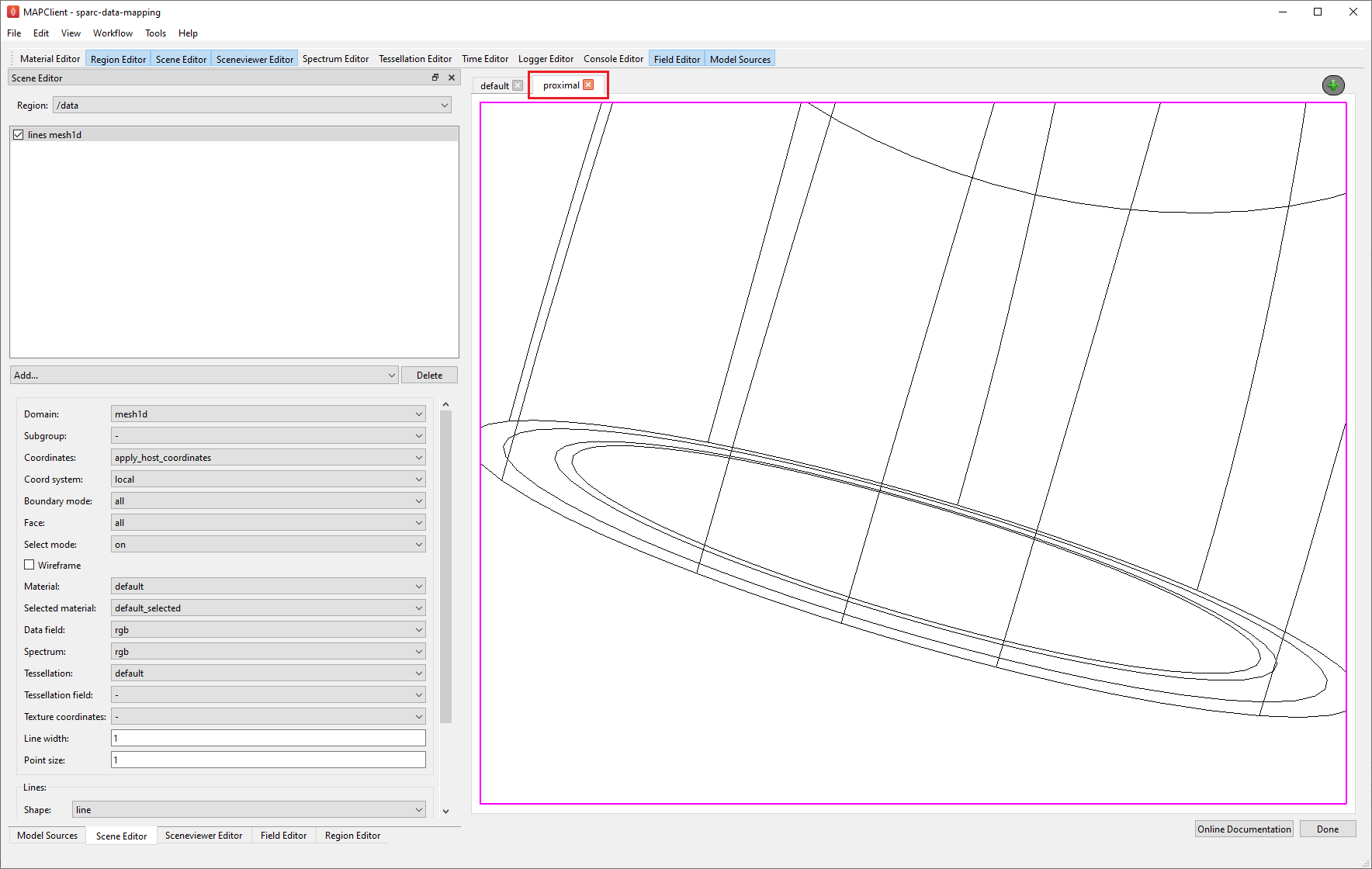
Go back to the / region and re-check the lines to show the colon surface again. Use the sceneviewer editor's View All button and zoom and translate the scene so that the proximal colon comes into view and the embedded data is as well.

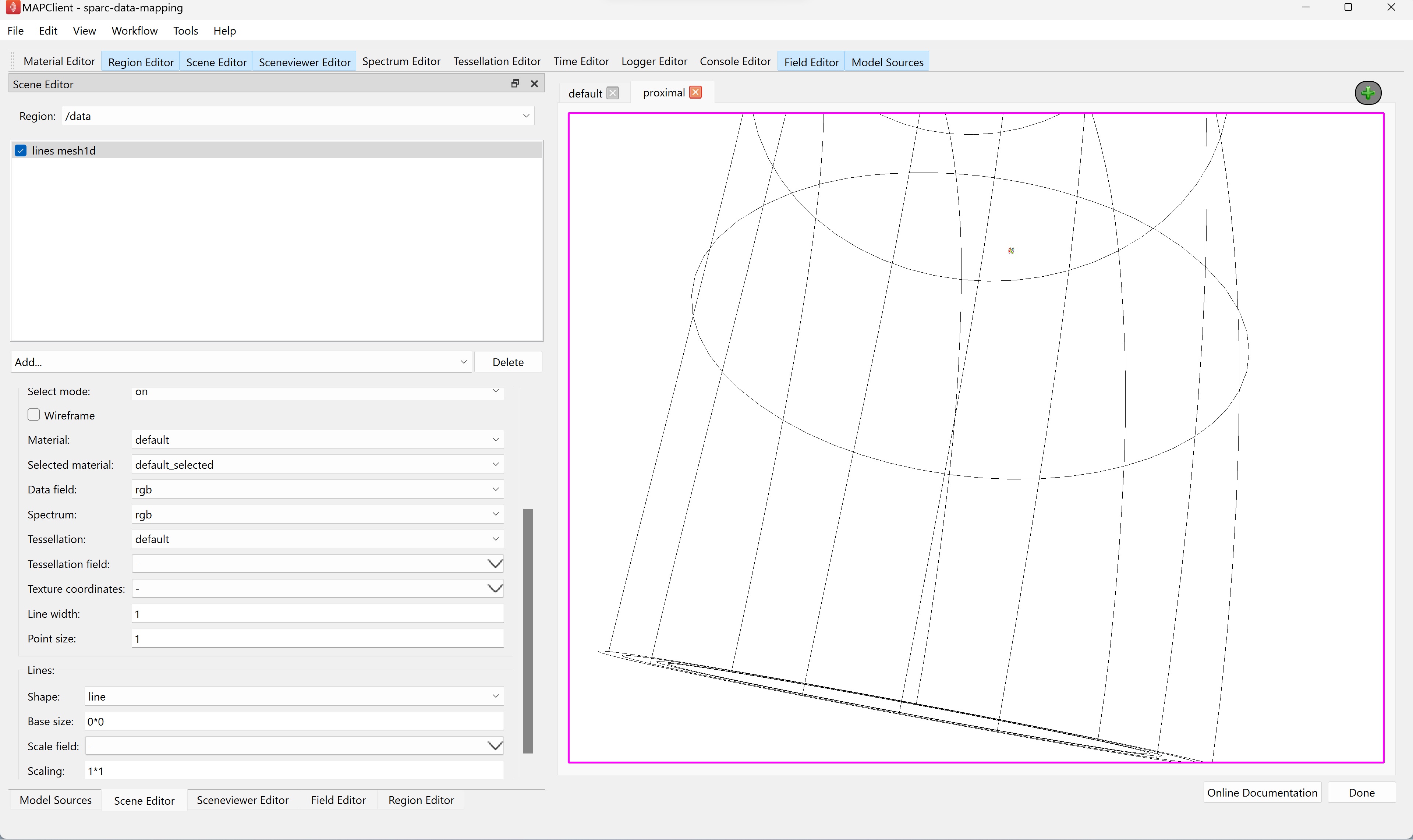
With this done we have now created two views -- the default view showing the whole mouse colon (and the segmented data but this is practically invisible due to scale), and the proximal view zoomed in to show the digital tracing of the enteric plexus which we embedded in the mouse colon scaffold.

Next, we will try and jazz up the visualization by adding a translucent purple surface to the scaffold.

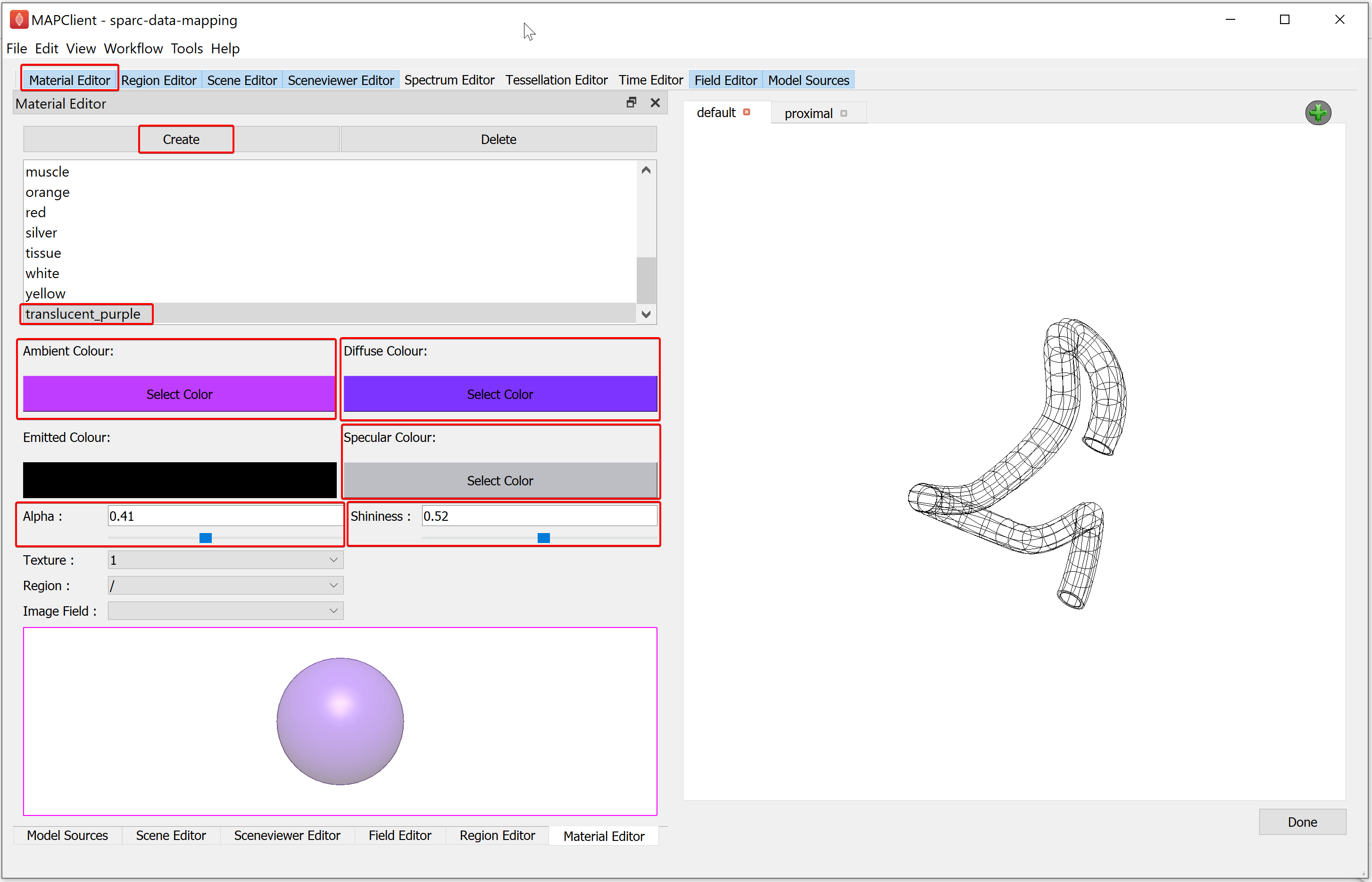
To create the translucent purple material, we use the Material Editor. In the Material Editor window create a new material called translucent_purple. Select the Ambient Colour to a light shade of purple, the Diffuse Colour to a darker shade of purple than used for the ambient colour, and the Specular Colour as a light grey. And set the Alpha and Shininess values to 0.41 and 0.52 respectively.

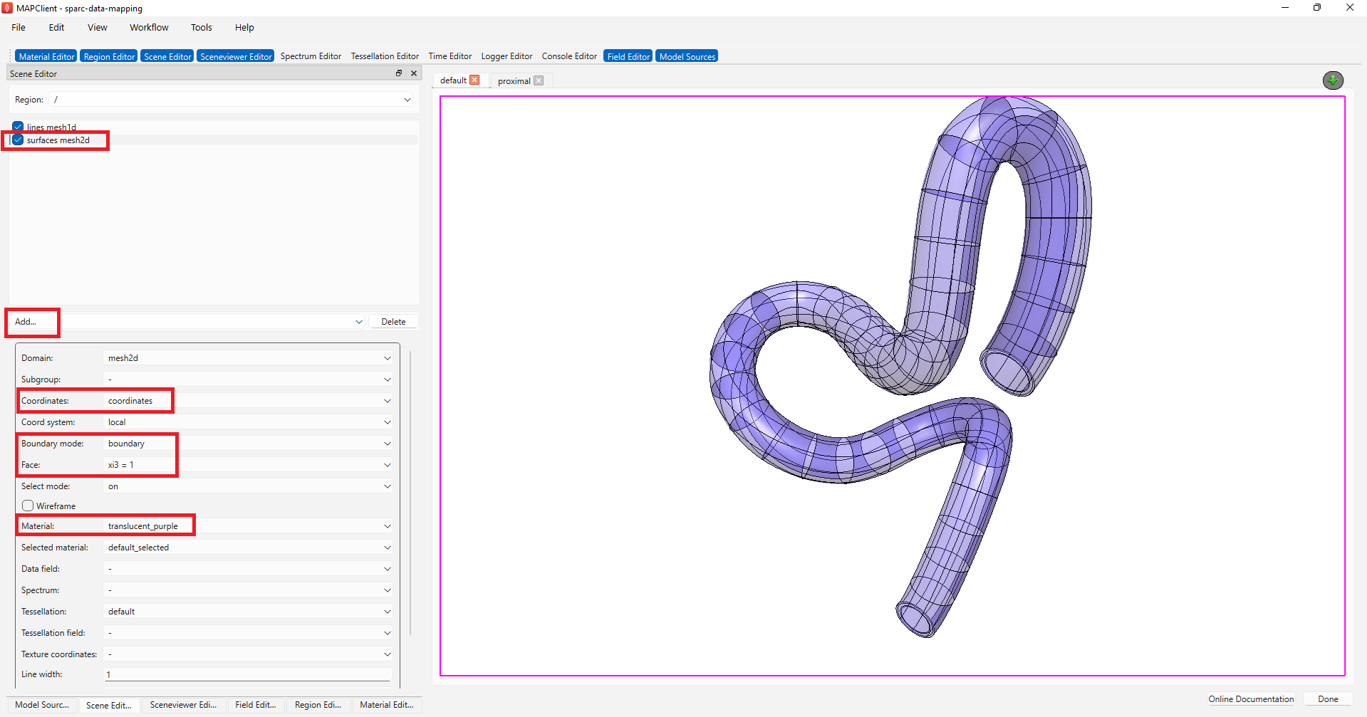
Now we will create some surface graphics that use the translucent material we have just created. With the Scene Editor, set the Region chooser to the root region (/). Use the Add graphics chooser to add a surface graphic, set the Coordinates value to coordinates, select the Boundary Mode to boundary, Face value to xi3 = 1, and set the Material option to translucent_purple.

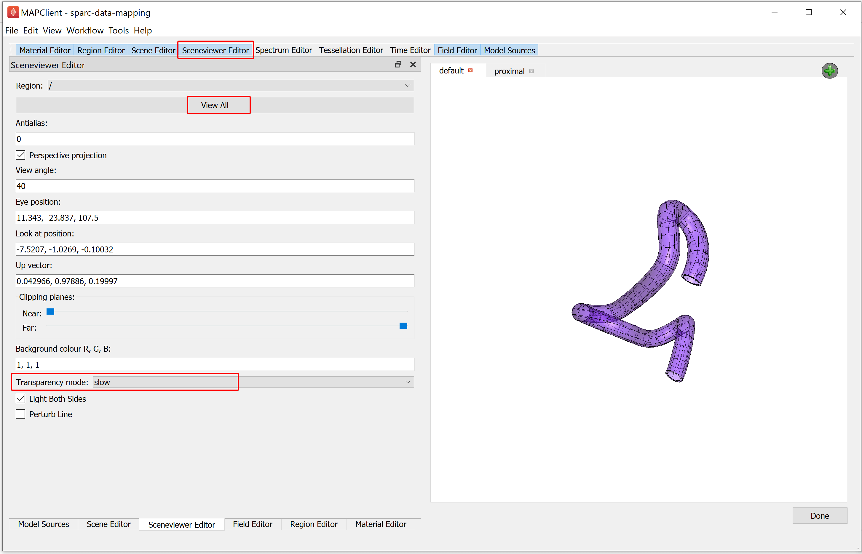
When we use transparent surfaces, we often see undesirable visual artifacts. This is because we are using a simplistic calculation for which surface is in front of another. We can change this behavior by changing the Transparency mode. The Transparency mode can be modified using the Sceneviewer Editor. Using the Sceneviewer Editor, change the Transparency mode to slow and click on the View All button to view the segmented data.

Manipulate the scene to show the best viewing point to finish. When you are satisfied that you have the best viewing point click on the Done button.

The last three steps in the workflow generate the outputs for the SPARC dataset. These steps create the scaffold annotations file, the webGL export of the visualization, and the thumbnail for the visualization. These three steps are non-interactive and no interface is shown for them. It should be noted that these steps can take a small amount of time before they finish processing. When the exports have been saved the user interface will show the workflow as it was when we started executing.

Once the workflow has finished executing (returned to its initial state), navigate to the derivative folder (DATASET_ROOT\derivative\scaffold) to view the output files. For the example above, some of the output files are as follows:

1. mouse_colon_metadata.json is the webGL export of the visualization, file used for displaying visualization on the portal.

2. mouse_colon_default_view.json and mouse_colon_default_thumbnail.jpeg are the view file and thumbnail file associated with the default view.

3. mouse_colon_proximal_view.json and mouse_colon_proximal_thumbnail.jpeg are the view file and thumbnail file associated with the proximal view.

4. OrganScaffold_annotations.csv file contains the scaffold annotations.

Move on to annotating or return to the main Scaffold Mapping Tools page.