Scaffold Mapping Tools: Mapping Physiological Data
How to map physiological data to a scaffold
In this demonstration, we are going to work through how to map physiological data to an organ scaffold.
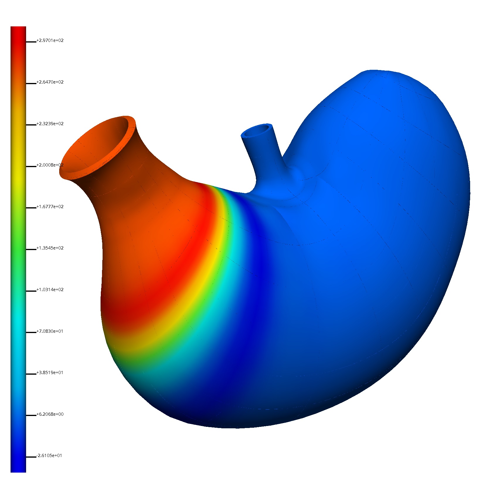
Table of Contents
- Setup
- Prepare Workflow
- Embed the SPARC Data in a Scaffold
- Visualize the Mapped SPARC Data on a Scaffold
NoteThis documentation is written for the latest version of the mapping tools. Previous versions of this documentation are available.
Older versions of this documentation:
Setup
First, we need to create a skeleton dataset as defined here.
Second, we download the physiological data. A copy of which is given below for reference.
CSV data
| pyloric antrum | body of stomach | |
| ghr | 45.9 | 69.3 |
| som | 104.7 | 50.8 |
| gas | 274.1 | 2.4 |
| 5ht | 67.7 | 13.6 |
| hdc | 50.8 | 298.2 |
| pyy | 26.4 | .2 |
Table 1: Cell density information.
Download the cell density data file and save it in the primary directory of the skeleton dataset created above; we will use this file in our workflow.
Prepare Workflow
Step 1: Launch MAP Client Mapping Tools
Launch MAP Client Mapping Tools, found in the Start Menu under MAP-Client-mapping-tools vX.Y.Z (The X, Y, and Z will be actual numbers depending on the current stable release).
If you don't yet have the MAP Client Mapping Tools available, follow the instructions here.
Step 2: Create a workflow
Create a new workflow on the Desktop. Using Windows explorer, or similar, create a new directory on the Desktop and name it cell_density_map.
From the File menu in MAP Client Mapping Tools select the New workflow (CTRL-N) to start a new workflow. Navigate to the Desktop and select the cell_density_map directory created earlier.
Now that we have a fresh workflow we can construct a workflow to map the physiological data. To construct the workflow we will drag steps from the step list box onto the workflow panel and connect the steps together.
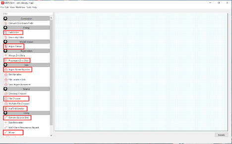
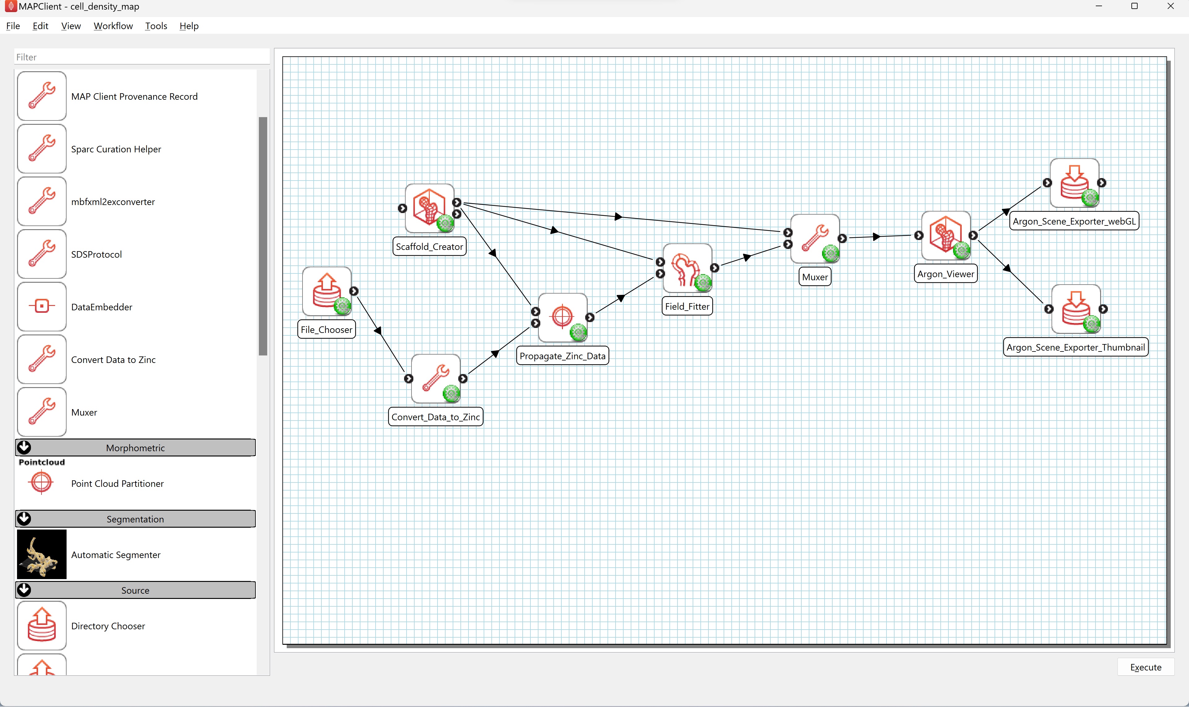
We will use the following steps which can be found in the step list box on the left-hand side of the main window (Figure 1).
- File Chooser
- Field Fitter
- Argon Viewer
- Propagate Zinc Data
- 2 x Argon Scene Exporter
- Scaffold Creator
- Convert Data to Zinc
- Muxer
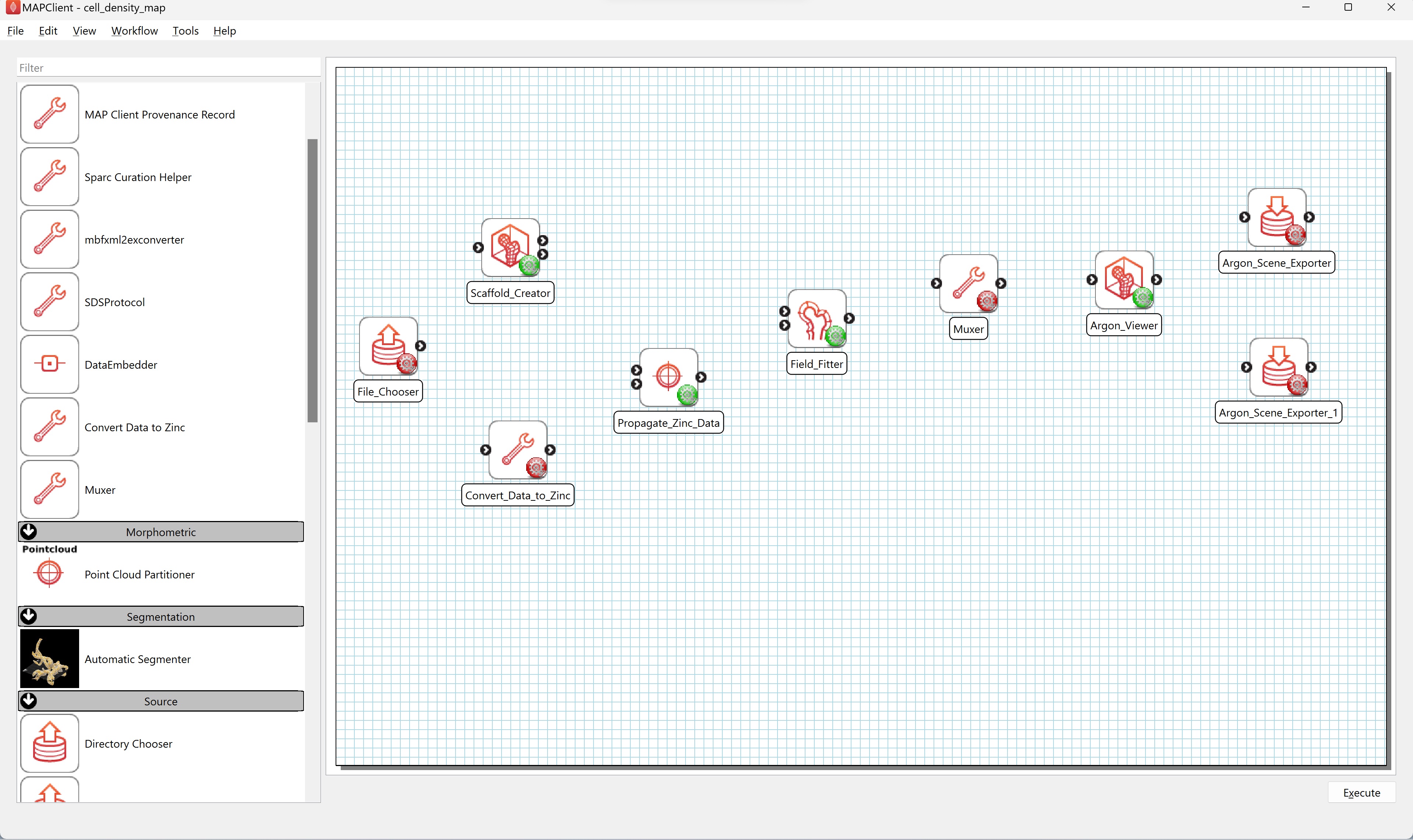
Drag these steps from the step list box onto the workflow panel.
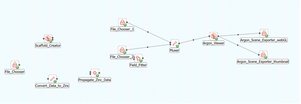
Layout the steps as follows (see Figure 2):
The File Chooser step and Scaffold Creator steps are source steps and should be placed on the left hand side of the workflow panel. The Scaffold Creator should be placed above the File Chooser step. The Convert Data to Zinc step should be placed to the right of the File Chooser step. The Propagate Zinc Data step is placed to the right of the Convert Data to Zinc step. The Field Fitter step is placed to the right of the Propagate Zinc Data step and vertically in the middle of the Scaffold Creator step and the File Chooser step. The Muxer step is placed to the right of the Field Fitter step. The Argon Viewer step is placed to the right of the Muxer step. Two Argon Scene Exporter steps are placed to the right of the Argon Viewer step, placed one above the other vertically.
Step 3: Configure the Workflow
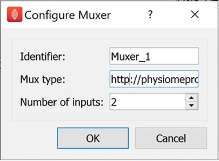
Now we configure all the steps in the workflow that are showing red configure icons. We will start with the Muxer step.
The Muxer step requires two parameters to be configured. The Mux type parameter and the Number of Inputs parameter. The Mux type parameter should be given the value: http://physiomeproject.org/workflow/1.0/rdf-schema#file_location. The Number of Inputs parameter should be set to 2.
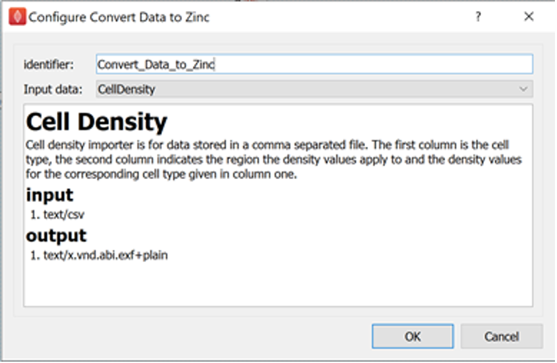
Next we configure the Convert Data to Zinc step. The Convert Data to Zinc step has one parameter to configure, that is the Input data parameter. For the data we are working with, the Input data parameter should be set to CellDensity.
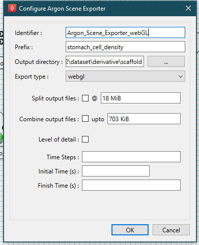
Next, configure the two Argon Scene Exporter steps. Configure the identifier of one of these steps to be Argon_Scene_Exporter_webGL. Configure the identifier of the other Argon Scene Exporter step to be Argon_Scene_Exporter_thumbnail. For the Argon Scene Exporter step with identifier Argon_Scene_Exporter_webGL set the prefix parameter to stomach_cell_density, the export type parameter to webgl, and set the output directory to the derivative directory of the skeleton dataset created earlier. We can create a scaffold directory under the derivative directory to use as the output directory, if we wish.
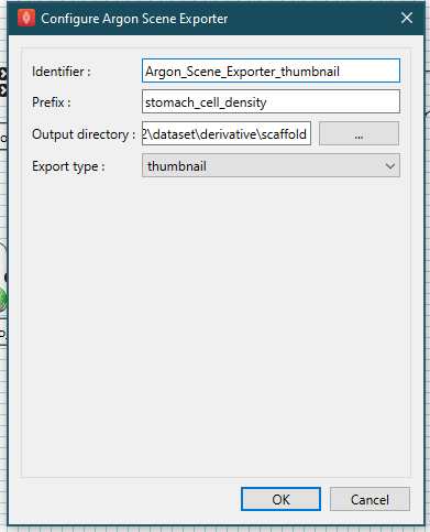
For the Argon Scene Exporter step with identifier Argon_Scene_Exporter_thumbnail set the prefix parameter to stomach_cell_density, the export type parameter to thumbnail, and set the output directory to the derivative directory of the skeleton dataset created earlier. We can create a scaffold directory under the derivative directory to use as the output directory, if we wish.
Best practice is to set the output directory of the thumbnail to the same directory as the webGL.
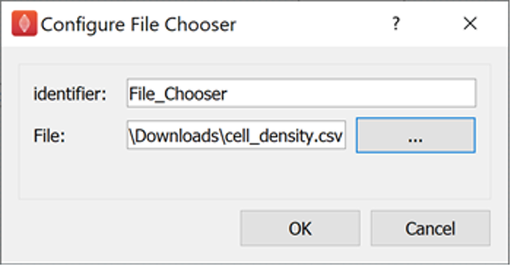
The last step to configure is the source data to map; here we are mapping cell density data.
The cell density file we created from Table 1 is the source data we are going to map.
Configure the file parameter of the File Chooser step to be the cell_density.csv file.
The next stage in creating the workflow is to connect the steps.
The connections are as follows (see Figure 8).
- File Chooser connects to Convert Data to Zinc
- The first provides port of Scaffold Creator connects to
- the first uses port of Propagate Zinc Data
- the first uses port of Field Fitter
- the first uses port of Muxer
- Convert Data to Zinc connects to the second uses port of Propagate Zinc Data
- Propagate Zinc Data provides port connects to the second uses port of Field Fitter
- Field Fitter provides port connects to the second uses port of Muxer
- Muxer connects to the uses port of Argon Viewer
- Argon Viewer provides port connects to
- Argon Scene Exporter webGL
- Argon Scene Exporter thumbnail
Save the workflow.
At this point the workflow has been created and is ready for executing.
Step 4: Execute workflow
Execute the workflow press the Execute button in the lower right corner of the application main window (keyboard shortcut CTRL-X).
Embed the SPARC Data in a Scaffold
Step 1: Select a Scaffold
Using the Scaffold Creator interface set the Scaffold type to 3D Stomach 1. Set the Parameter set to Rat 1. The generation of the stomach scaffold may take 5-10 seconds to generate. Use the View All and Std. Views button to centre the generated scaffold in the viewing panel.
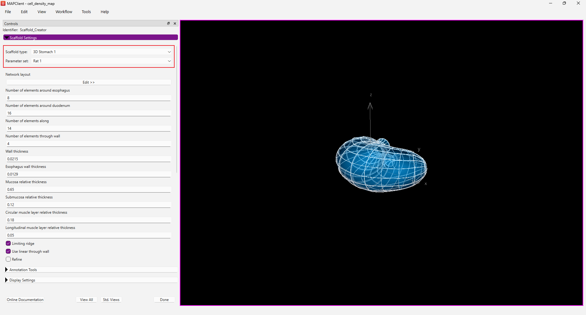
Click the Done button to finalise the settings and move onto the next step in the workflow.
Step 2: Fitting physiological data
The next visual step in the workflow is the Field Fitter step.
In this step we fit the fields available to us that we have converted from the cell density data and propagated over the appropriate stomach region.
Select the six cell density fields for fitting in the Fit Fields panel.
The six fields we select for fitting should be:
- 5ht
- gas
- ghr
- hdc
- pyy
- som
Set the Gradient 1 penalty to 0.001 to constrain the fit.
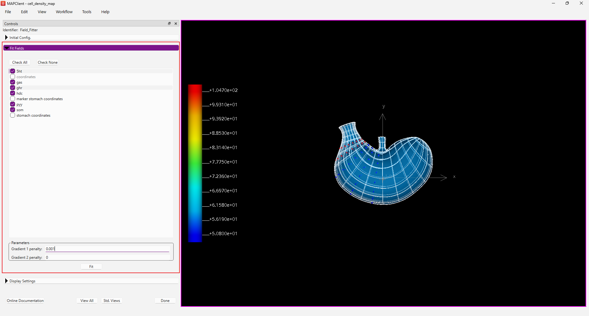
Click the Done button to do the fit, finalise the settings, and move onto the next step in the workflow. Alternatively, you can use the Fit button to do the fit before finalising the settings and display the result of the fit before moving to the next step if desired. The fitting process for this data takes about 8 seconds per cell density, and on a reasonable computer will take about a minute all up.
Visualize the Mapped SPARC Data on a Scaffold
Step 1: Adding a View
This first step in creating the visualisation is add a view. Click on the the Add View button on the main widget.
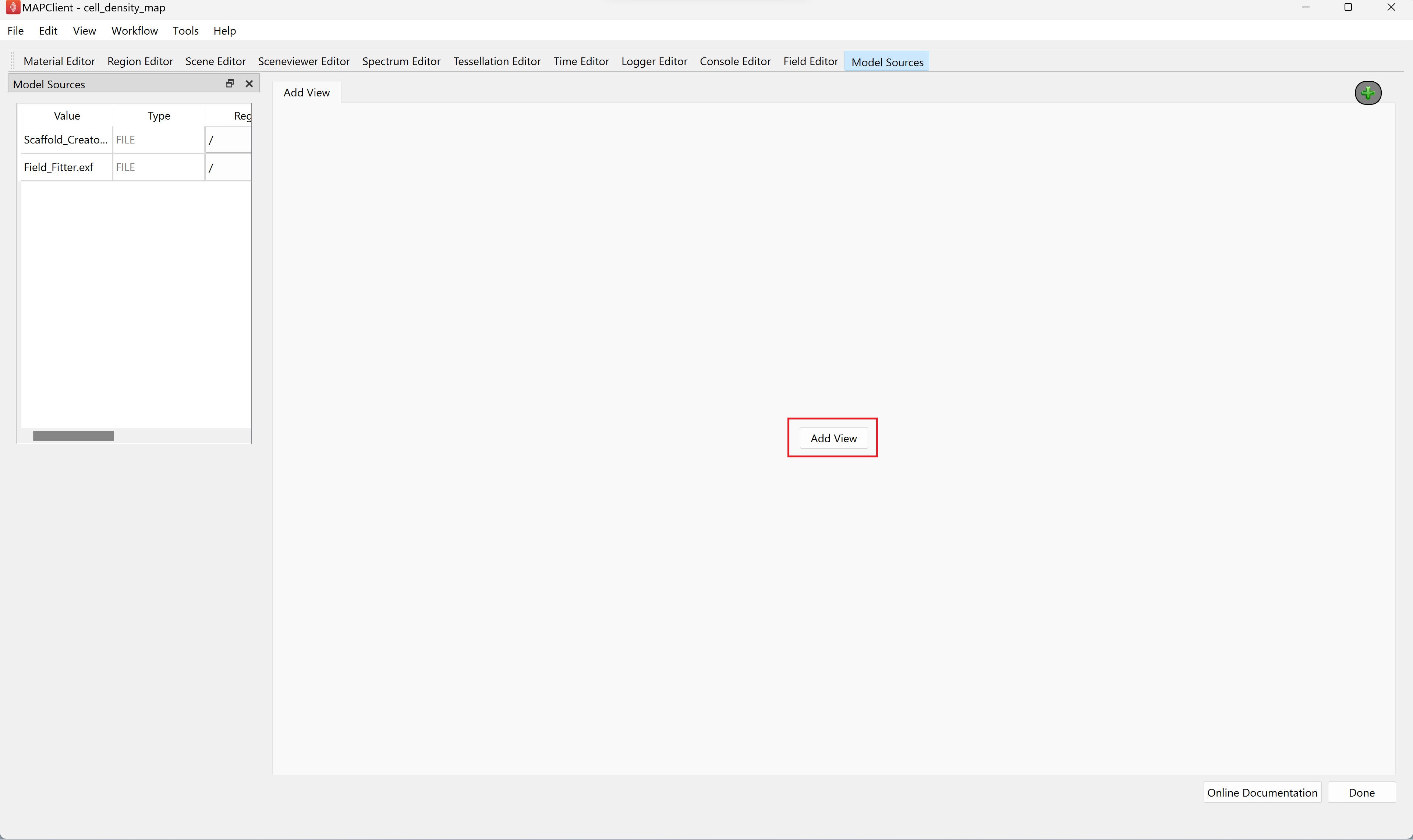
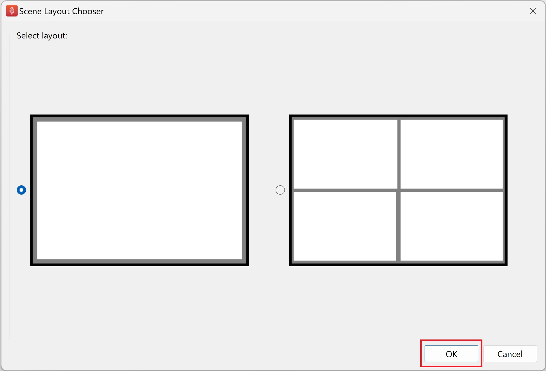
In the Scene Layout Chooser dialog that appears click the Ok button to choose the default single view layout option.
Rename the view by double clicking on the tab header text, currently named Layout1 and rename it to default.
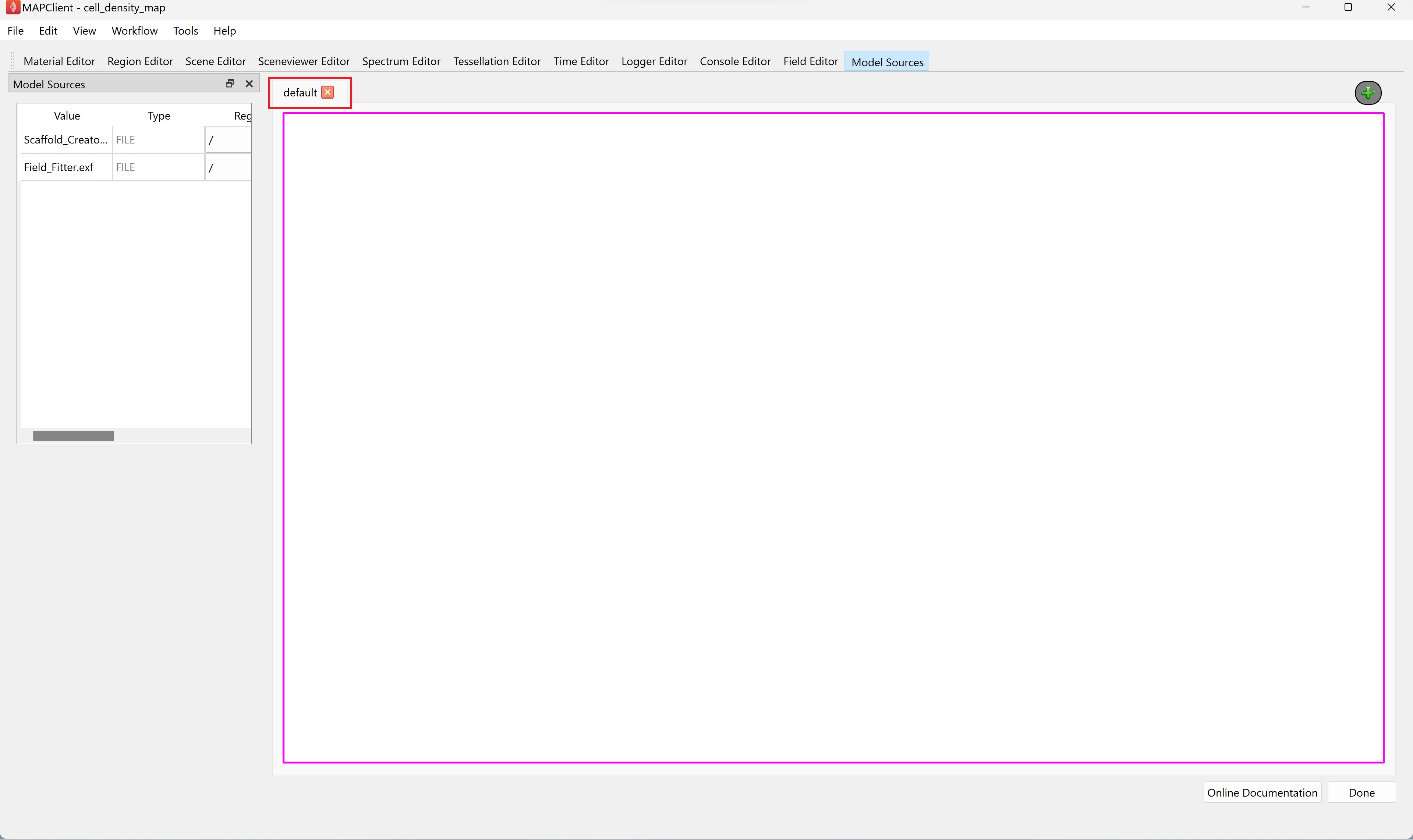
Step 2: Load Model Sources
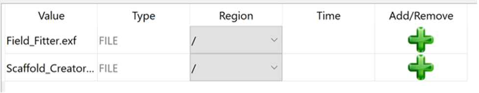
Use the Model Sources editor to load both the input data files into the root (/) region. Click on the green plus

button to apply the associated source to the region specified in the region column.
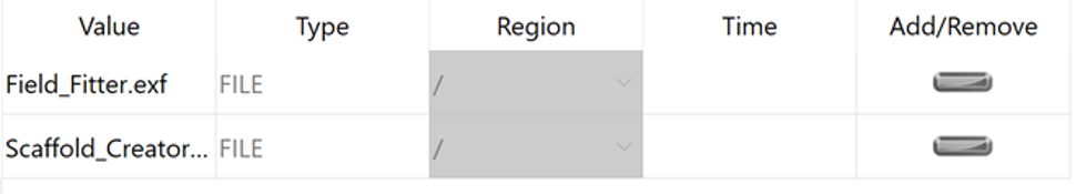
When the model sources are applied the Add/Remove column will show a grey minus symbol:
Step 3: Visualizing
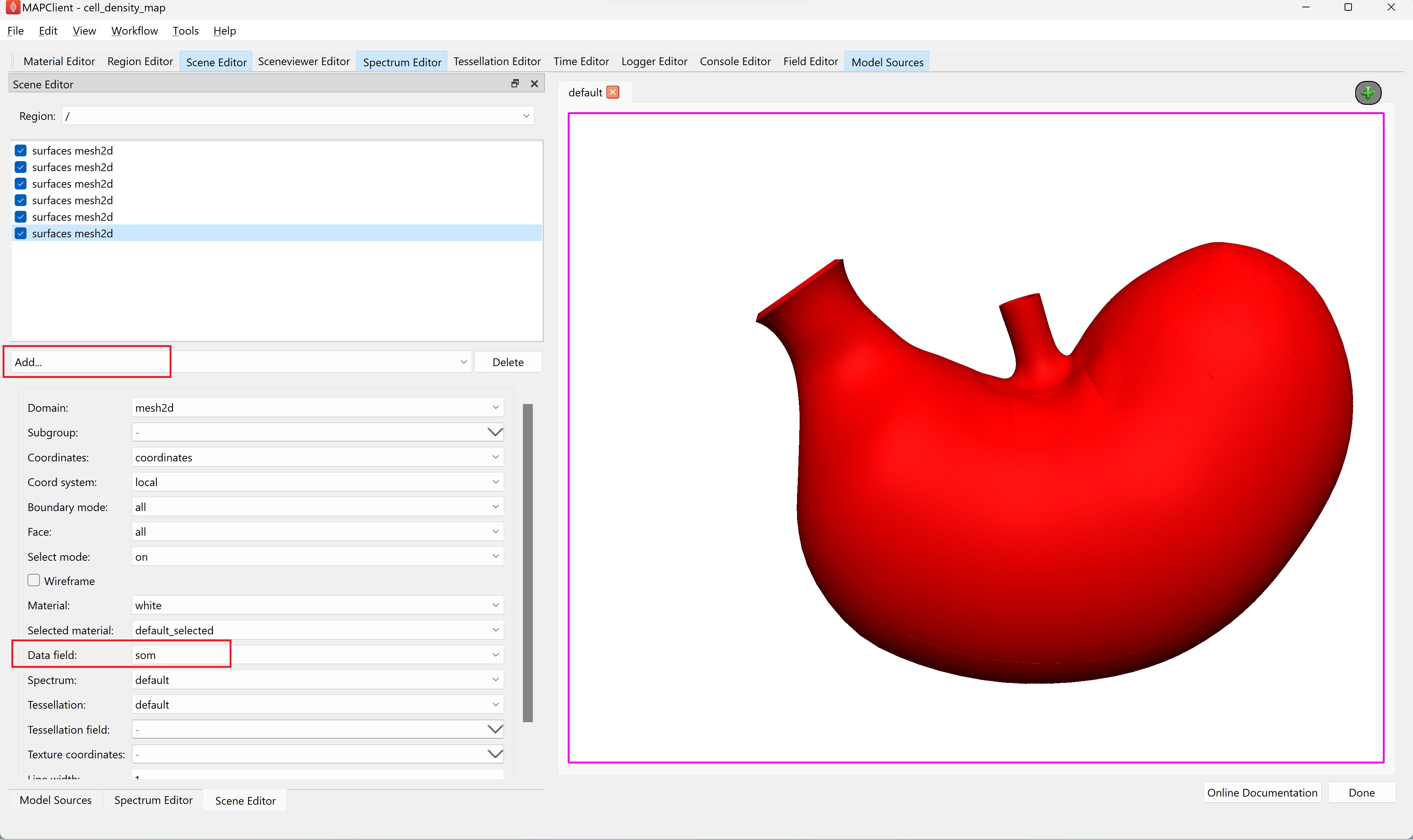
Switch to the Scene Editor to add graphics that will display the scaffold and the fitted data. Add six surface graphics, one for each cell density field, using the Add… graphics chooser. For each surface graphic set the Data field to a cell density field (one of; 5ht, gas, ghr, hdc, pyy, som).
Once all six surfaces have a unique cell density field set, use the Spectrum Editor widget to autorange the default spectrum to all fields currently using the spectrum.
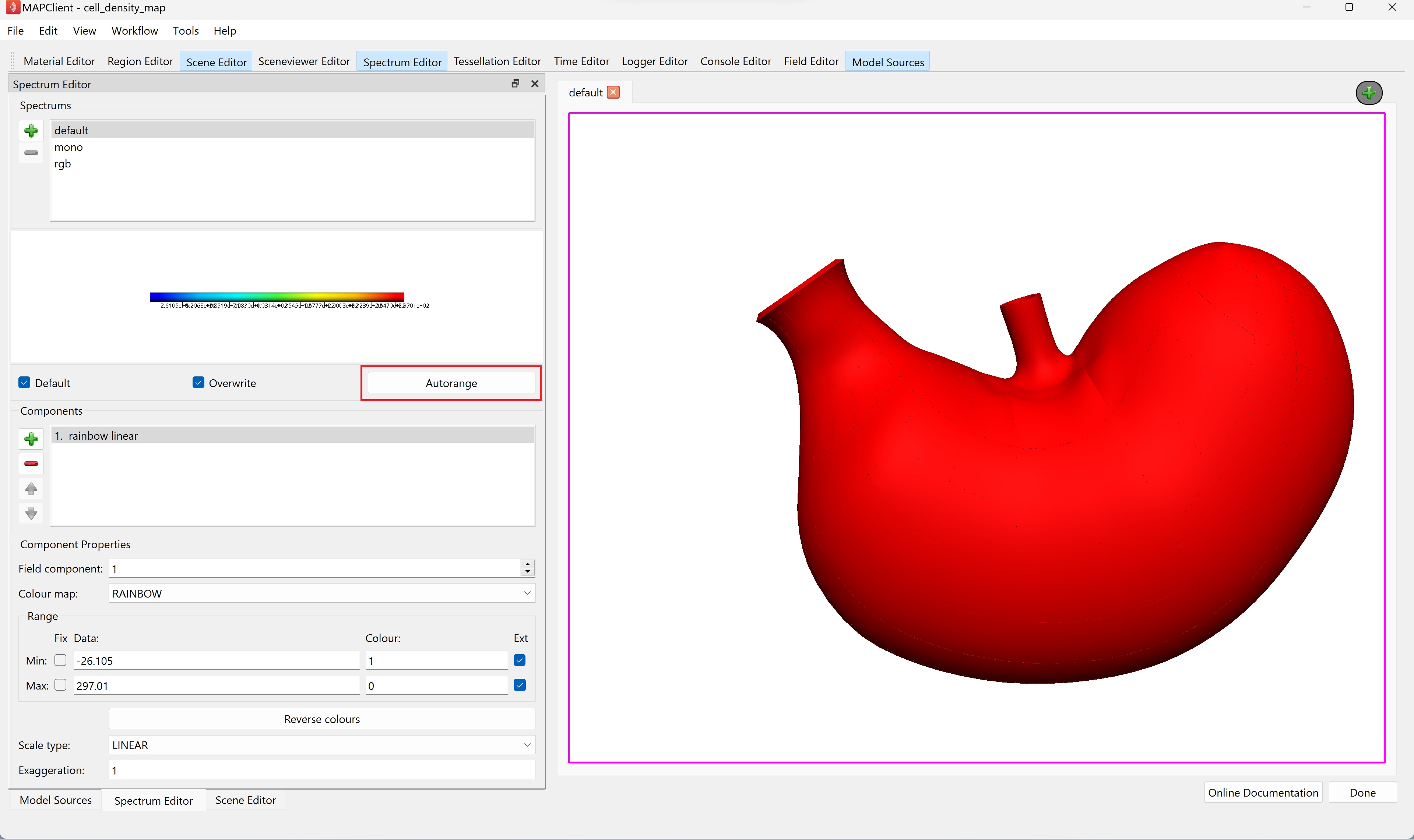
NoteWe need to have all added surfaces with the correct cell density field visible (checked) before autoranging the spectrum. If this is not then the autoranging will only be done over those surfaces that are visible and using a data field.
Step 4: Preparation for Export
Use the Sceneviewer Editor to adjust the view to show the whole scaffold, we do this by clicking the View All button. The last task is to create a visualisation that we want to export into the webGL format.
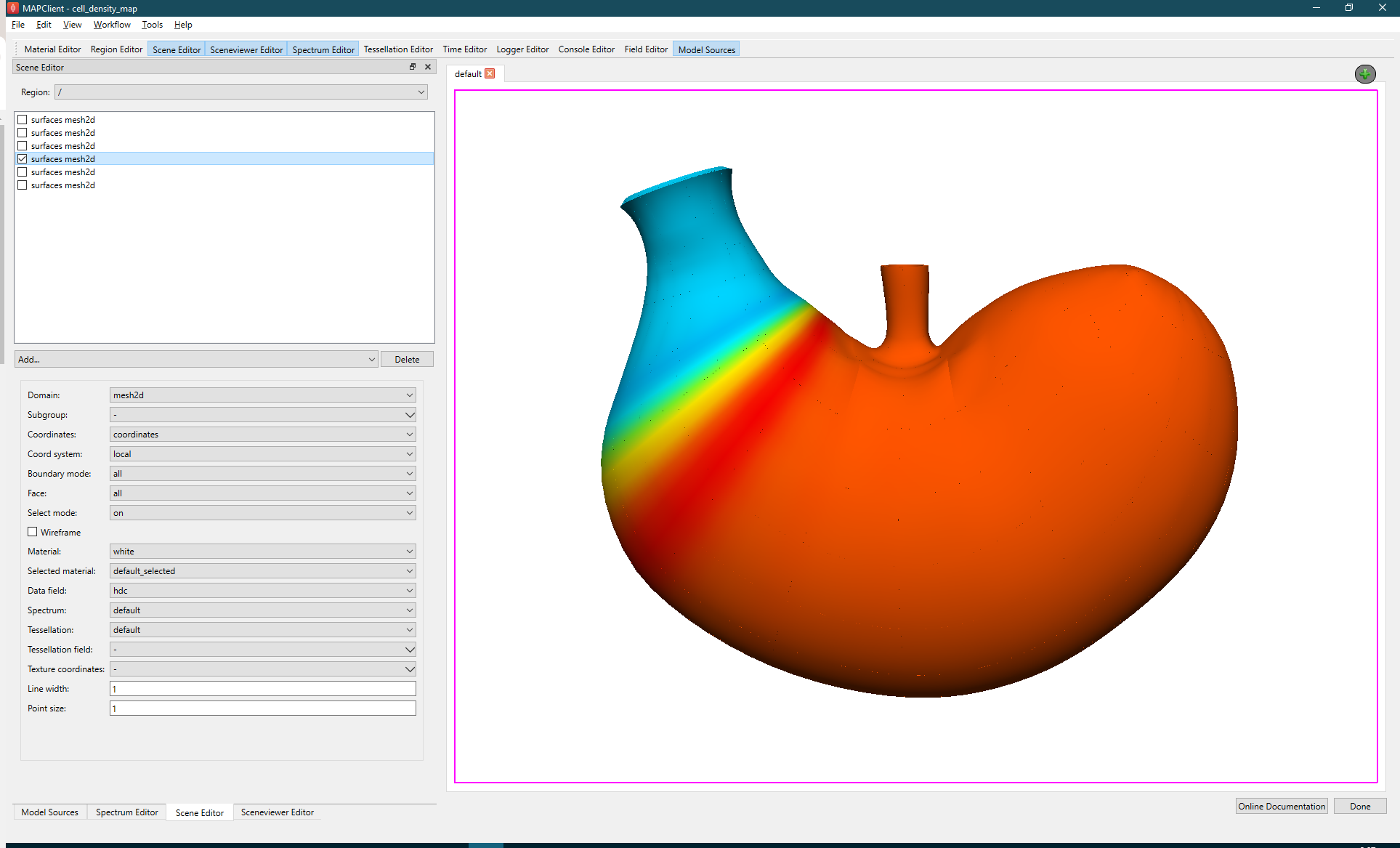
Deselect all surface graphics in the Scene Editor and then select only one, the surface visualisation that shows the data to best effect (see Figure 16).
To export the finished visualisation click the Done button. Once the webGL and thumbnail have been generated, this will take a few seconds 5-10 typically, the workflow will finish and return to the view of the workflow panel.
Special Note
If we wanted to create webGL output for all the cell densities it would be tiresome to go through this whole process five more times. We can shortcut this process by editing the current workflow. This can be done by adding two File Chooser steps and removing all the connections leading into the Muxer step. We could then connect the two File Chooser steps into the Muxer, select the Scaffold_Creator.exf file from inside the workflow directory for the first File Chooser and select the Field_Fitter.exf file from inside the workflow directory for the second File Chooser.
We could then create a new scaffold output directory within the skeleton dataset created at the start, direct the webGL and thumbnail export steps to use those directories and re-run the workflow.
Now when we run the workflow we only need to make changes to the visualisation. In this case we could simply change the surface graphics that are currently displayed. Following this process for each surface graphic and changing the output directory will significantly reduce the time it takes to produce webGL content for adding to a SPARC dataset and submission to the SPARC portal.
Move on to annotating or return to the main Scaffold Mapping Tools page.
Updated 11 months ago