Scaffold Mapping Tools: Mapping Image Data From Flat Preparation
How to map segmented image data from a flat mount preparation to a SPARC organ scaffold
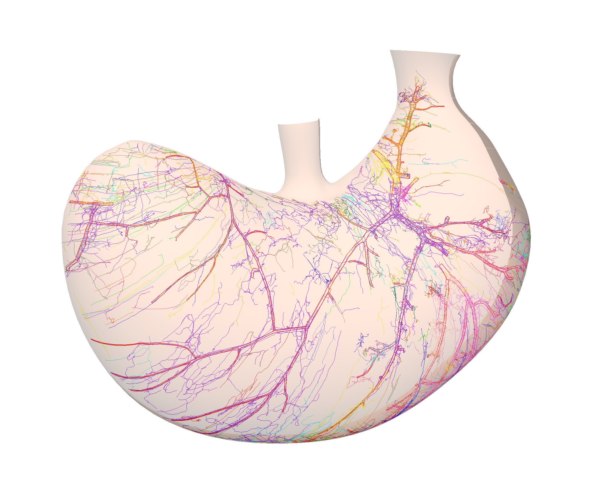
Table of Contents
- Setup
- Prepare Workflow
- Embed the SPARC Data in a Scaffold
- Visualize the Mapped SPARC Data on a Scaffold
NoteThis documentation is written for the latest version of the mapping tools. Previous versions of this documentation are available.
Older versions of this documentation:
Setup
First, we need to Create a Skeleton Dataset Structure.
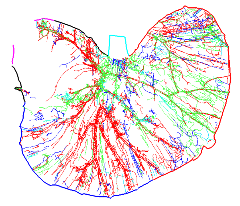
We will be using the segmentation from an image of a flat mount mouse dorsal stomach (Figure 1a, Courtesy of Zixi Cheng’s Lab, University of Central Florida) to demonstrate how to fit and map the calcitonin gene-related peptide (CGRP) immunoreactive innervation to a stomach scaffold.
NoteThe scaffold is annotated with standard anatomical names and terms (Figure 1b) as documented here. In order to fit the scaffold in later steps these terms are matched with similar terms from the segmented data. To follow this process for other sources of data, the data will need to have these annotations. There are tools available to add annotation terms to most forms of segmented data. For example, MBF Neurolucida tools.
In this example, we will be using a segmentation file that has been annotated with the necessary terms. Download the xml segmentation file to a local drive and we will use this file as our input file for the MBFXMLFile step in our workflow later.
Prepare Workflow
Step 1: Launch MAP Client Mapping Tools
Launch MAP Client Mapping Tools, found in the Start Menu under MAP-Client-mapping-tools vX.Y.Z (The X, Y, and Z will be actual numbers depending on the current stable release).
If you don't yet have the MAP Client Mapping Tools available, follow the instructions here.
Step 2: Create and execute a workflow
You can create a new workflow anywhere but here we will create one on the Desktop.
Using Windows Explorer, or similar, create a new directory on the Desktop and name it Flatmount Mapping.
From the File menu in MAP Client Mapping Tools select the New workflow (CTRL-N) to start a new workflow.
Navigate to the Desktop and select the Flatmount Mapping directory created earlier.
Follow the instructions here to configure the workflow and make sure you select the downloaded segmentation file as the input file instead for Step 1b).
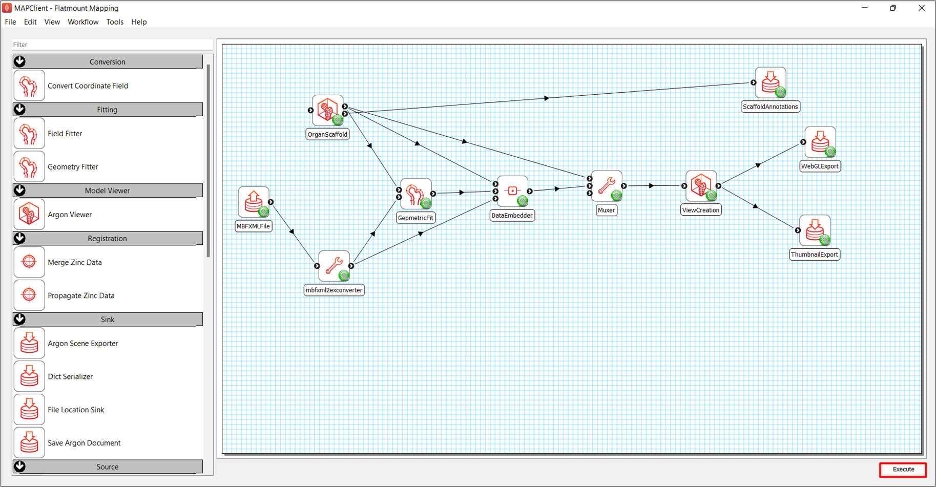
After setting up the workflow, as shown in Figure 2, save the workflow (keyboard shortcut CTRL-S) and execute the workflow by pressing the Execute button in the lower right corner of the application main window (or use the keyboard shortcut CTRL-X).
Embed the SPARC Data in a Scaffold
Step 1: Select a scaffold
At the Scaffold Creator interface, select 3D Stomach 1 under the Scaffold type and set the Parameter set to Mouse 1. The generation of the stomach scaffold may take 5-10 seconds.
Use the View All and Std. Views button to center the generated scaffold in the viewing panel (Figure 3).
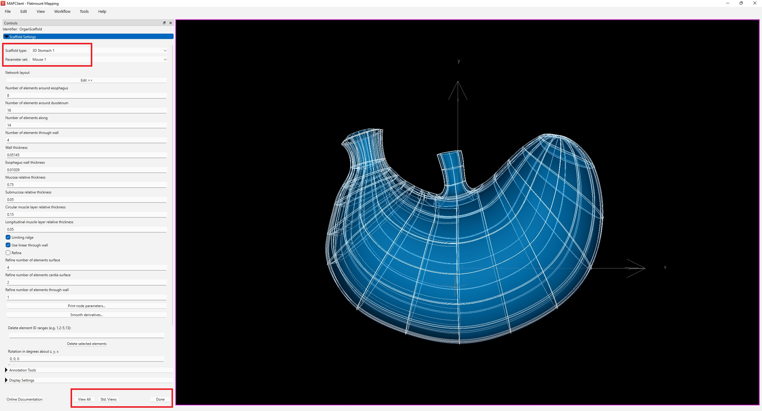
Click the Done button to finalize the settings and move on to the next step in the workflow.
Step 2: Fit the scaffold
The next visual step in the workflow is the Geometry Fitter step. Many of the config, align, and fit options in this step have "tool tips" which describe their use. These “tool tips” can be accessed by hovering the mouse pointer over an option.
Note: This documentation is a step-by-step guide customized for handling the example data. The fitting steps and their parameters used here have been specifically chosen to suit the example data. The fit can also be derived effectively with other combinations of fitting steps and their parameters. To achieve a desirable fit for your specific dataset, you may wish to refer to this documentation for a more detailed guide of the fitting process, techniques, steps, and parameter selection.
Config
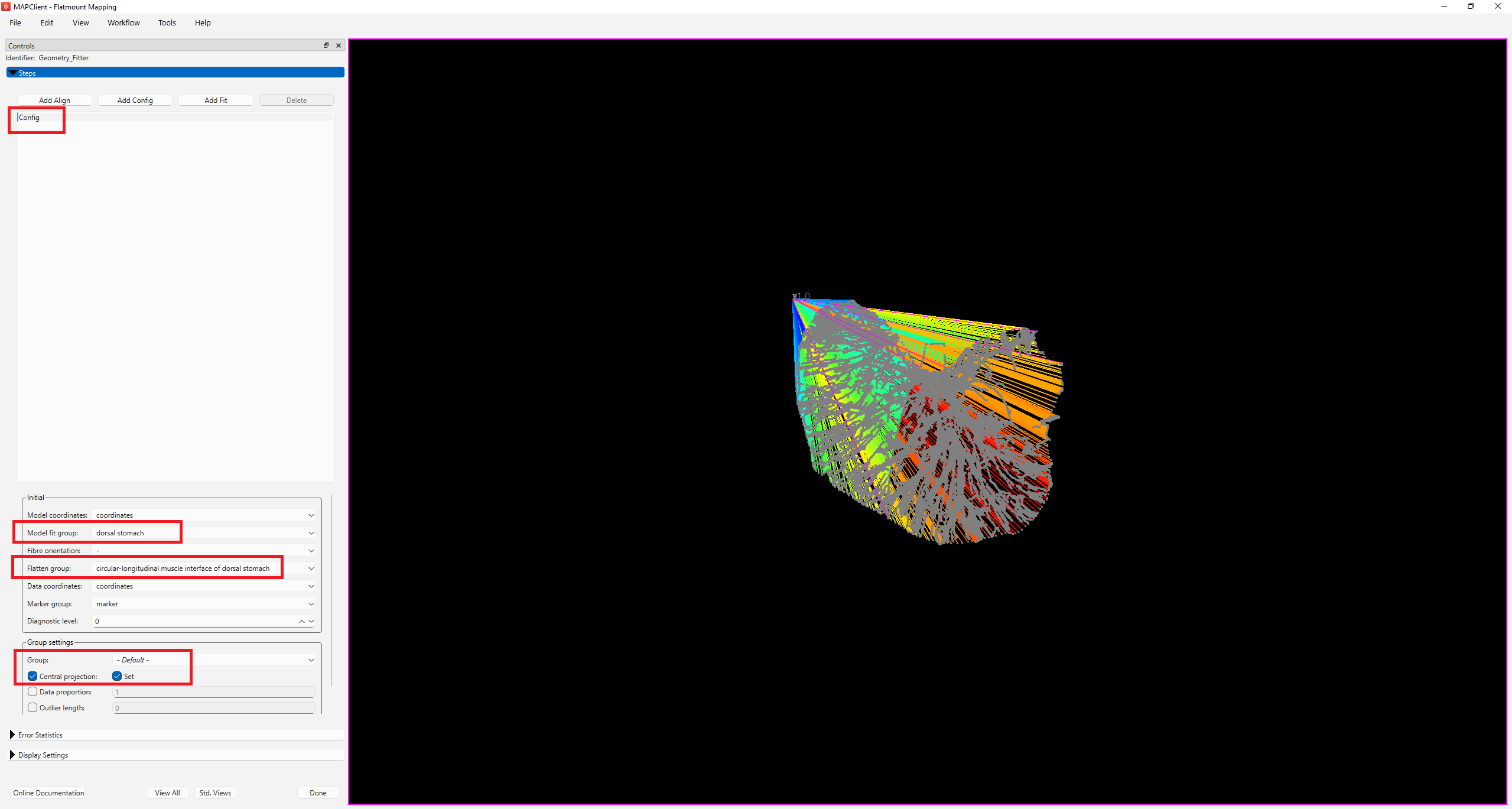
The first step is to set up the fitting parameters in the Config step (Figure 4). Given that this data is derived from a dorsal stomach sample, select dorsal stomach under the Model fit group as the group to be fitted.
Under Flatten group, select the group you wish to flatten. For the purpose of illustration in this example, we will map the CGRP data to the circular-longitudinal muscle interface of the dorsal stomach. Hence, select circular-longitudinal muscle interface of dorsal stomach under Flatten group.
Group settings control what data group is projected and how. Select -Default- under Group, and check the boxes next to Central Projection and Set. When set, the geometric center of the data and the scaffold group are calculated, and the data is projected as if these are at the same point; this is useful for early fitting steps where small features are not close to the data, but it must always be canceled later.
NoteCentral Projection can remain Set for certain groups where the span of data is likely to converge to the same result with it turned on or off (for example, inlet or outlet tubes). For these groups, Central Projection can remain Set for an extended period.
Align
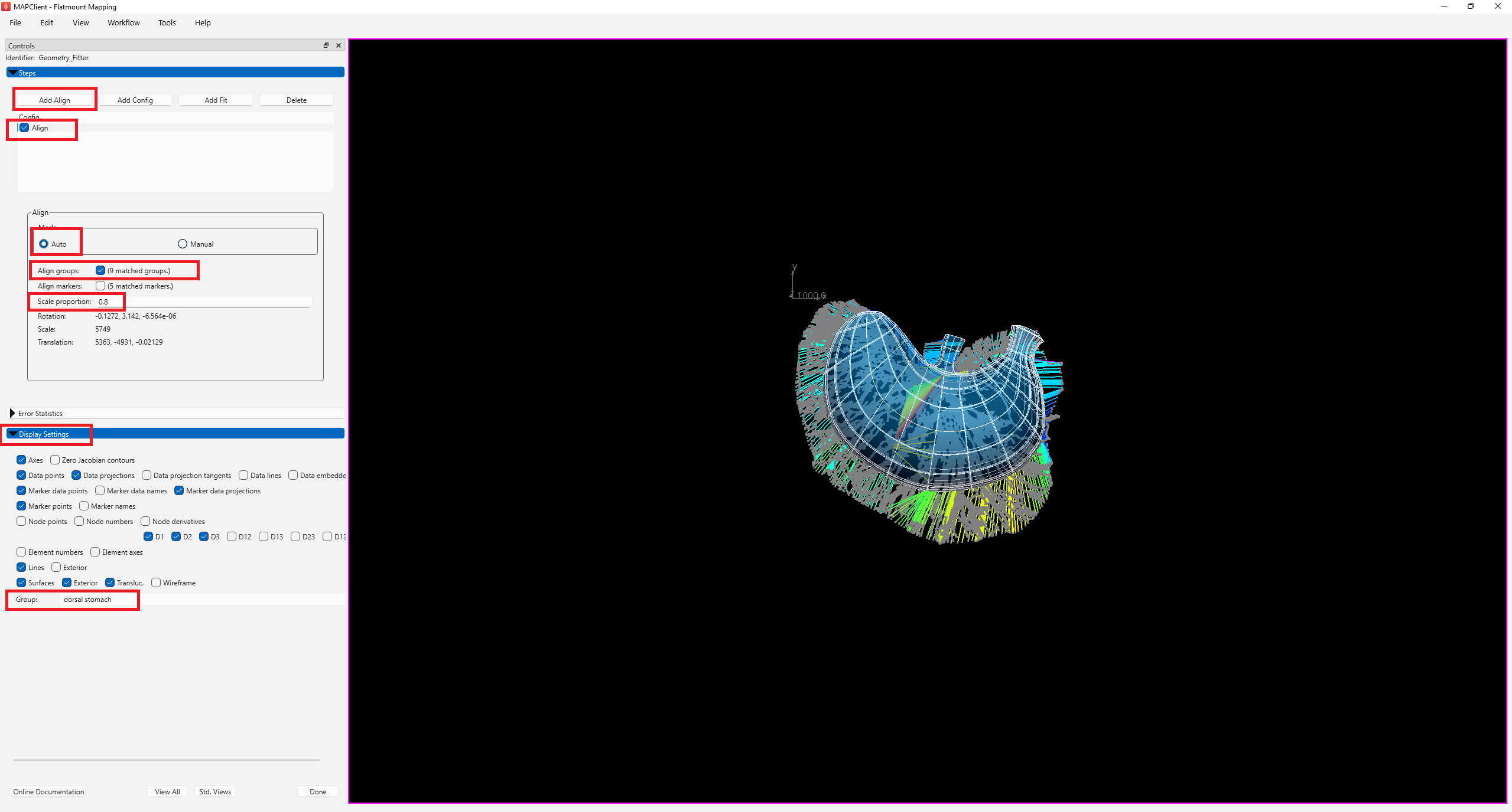
After the initial configuration, click Add Align button to add an alignment step. As the contour of the stomach data and mouse stomach scaffold both share common annotation terms, we can use Align groups to align groups of the same annotation on the data to the scaffold by selecting the Auto mode for alignment, then checking the box next to Align groups.
For this example, auto-alignment of the scaffold and data without scaling will result in an aligned scaffold that is still slightly bigger than the data contour. This is not ideal as it often results in undesirable fitting. To overcome this issue, set Scale proportion to 0.8. This will reduce the scaffold after auto-alignment by 0.8 times, and keep the scaffold within the data contour.
Under the Display settings, select dorsal stomach under Group. This feature allows visualization of the subgroup of the scaffold that is to be fitted.
Check the box next to Align on the Steps dialog box to invoke the alignment step (Figure 5).
Fit
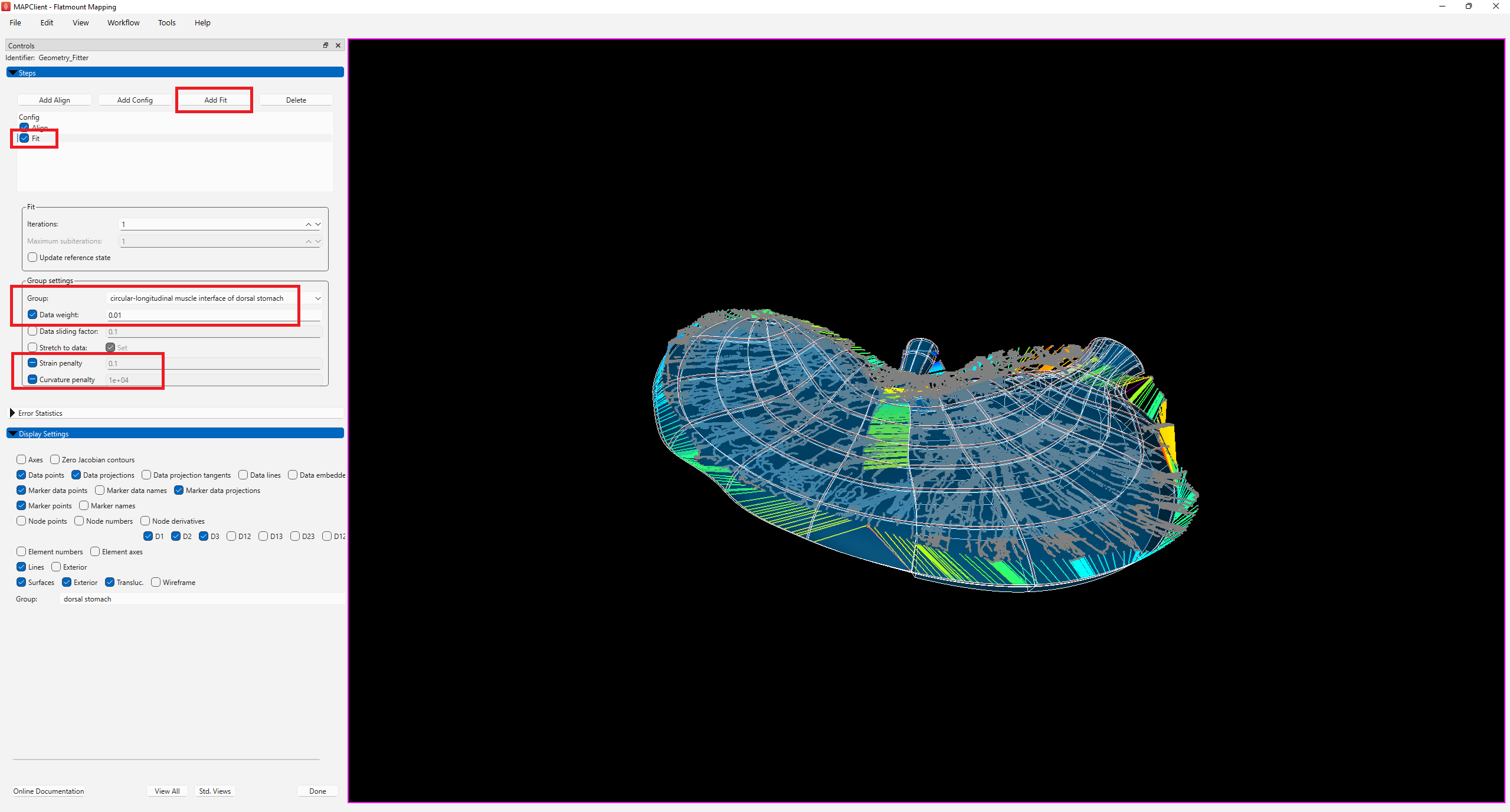
Now we are ready to start non-linear fitting, click on Add Fit to add a fit step.
For the -Default- group, check the box next to Strain penalty and set its value to 0.1, and set a Curvature penalty of 1e+04. Note that choosing these deformation penalty values takes experience, and some trial-and-error but generally it is recommended to start with a high strain penalty and curvature penalty, and lower the stiffness penalties gradually with more fits later in the process.
Under Group, change the selected term from -Default- to circular-longitudinal muscle interface of dorsal stomach, check the box next to Data weight and set the value to 0.01. As the circular-longitudinal muscle interface of dorsal stomach was chosen as the Flatten group under Config step, the Data weight for this chosen group now weighs the integral over that group which applies the flattening. Note that there should not be data points for the flatten group. A small value is usually selected initially and gradually increased over subsequent steps to avoid a wobbly flattening.
Click on the checkbox next to Fit in Steps to generate the fit (Figure 6).
As the fitted scaffold is now brought closer to the data, the central projection setting is no longer required. Click on Add Config to add a config step. Make sure that Group is set to -Default-, click on the box next to Central projection until you see a tick and uncheck the box next to Set.
Check the box next to Config under Steps to initiate the Config step (Figure 7).
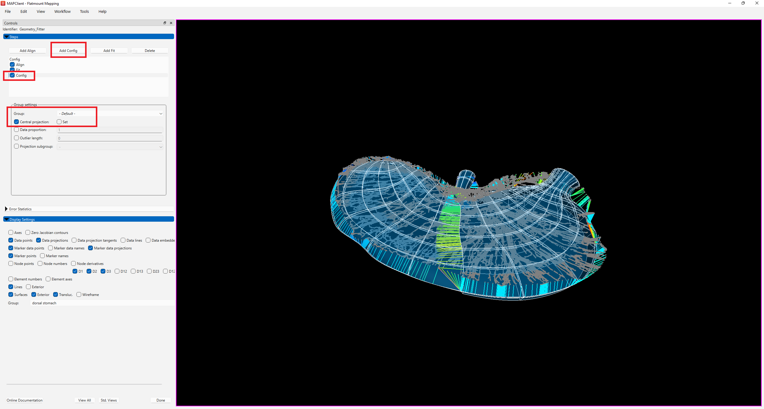
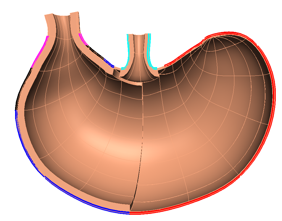
The fitted scaffold (Figure 7) has been flattened to some degree but is not completely flat at this stage. Nonetheless, the fit retains an ideal smooth distribution of elements across the scaffold. You will also notice that the scaffold fit overshoots data in some regions but that can be resolved with additional fitting steps by increasing the data weight for the flatten group and lowering deformation penalties.
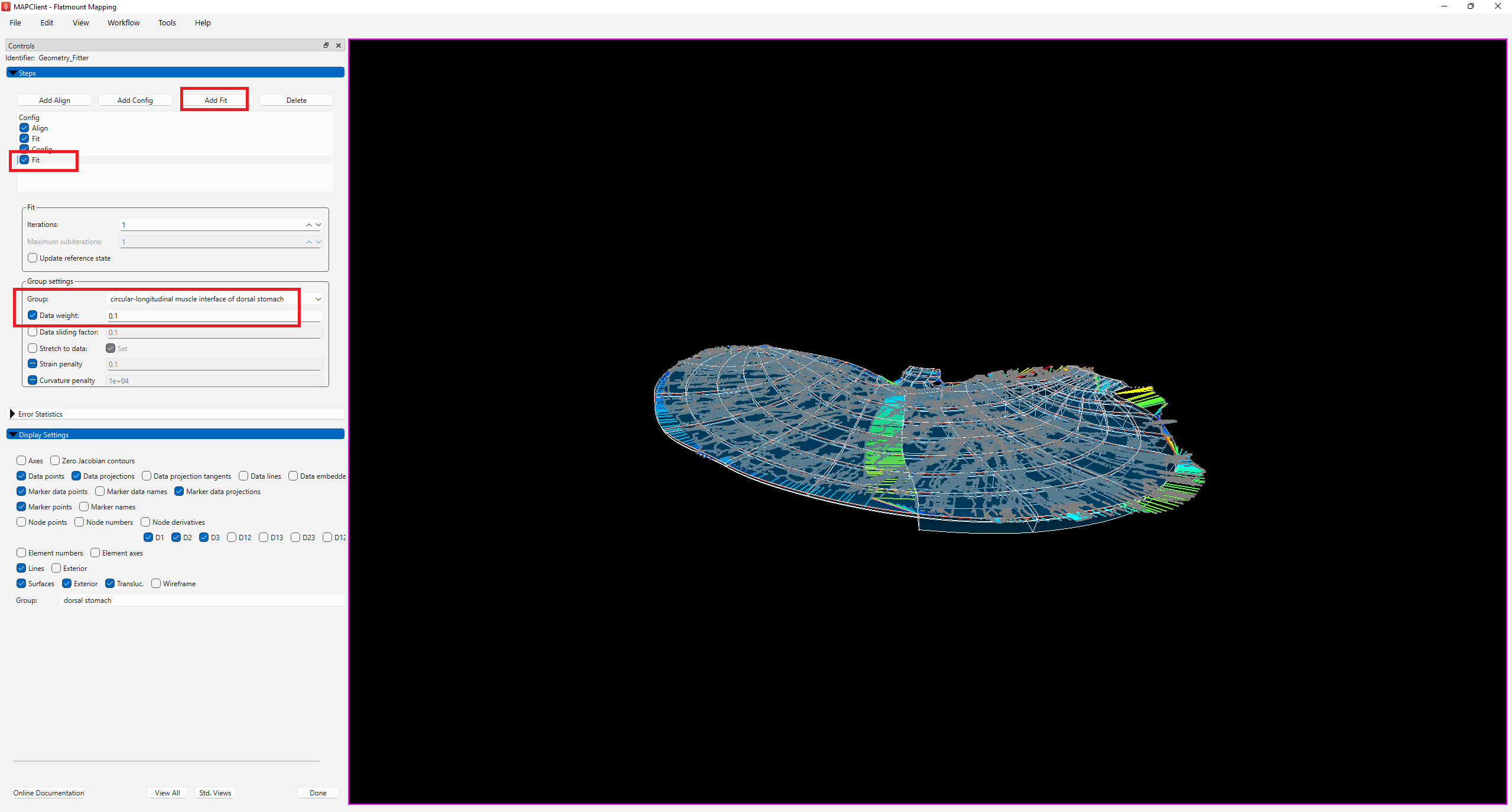
To do so, add another fit and lower the Data weight for circular-longitudinal muscle interface of dorsal stomach to 0.1. As demonstrated in Figure 8, the fit is now flattened.
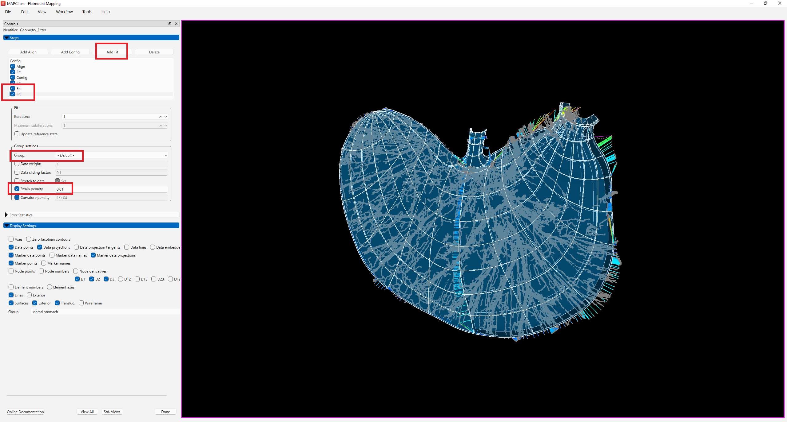
In order to bring the scaffold boundary closer towards the data contour, we add two new fit steps to reduce the Strain penalty of the -Default- group first to 0.05, and then to 0.01 to allow the gradual deformation of the scaffold to the data contour (Figure 9).
While the boundary of the scaffold is now closer to the data contour in most regions, it is noticeable that the data near the body, esophagus, pyloric antrum, and canal regions on the contour are still outside the scaffold. To improve the fit in these regions, we can add a new fit step and use the data weight of these groups to control the fit. Unlike data weight for the flatten group, data weight for the other non-flatten groups is a non-negative value which is usually used to make the selected group conform more closely to the data at the expense of other groups.
Click on Add Fit and under Group, toggle to the following groups and set their Data weight to 50:
- circular-longitudinal muscle interface of body of stomach along the gastric-omentum attachment
- circular-longitudinal muscle interface of esophagus along the cut margin
- circular-longitudinal muscle interface of pyloric antrum along the lesser curvature
- circular-longitudinal muscle interface of pyloric canal along the greater curvature
- circular-longitudinal muscle interface of pyloric canal along the lesser curvature
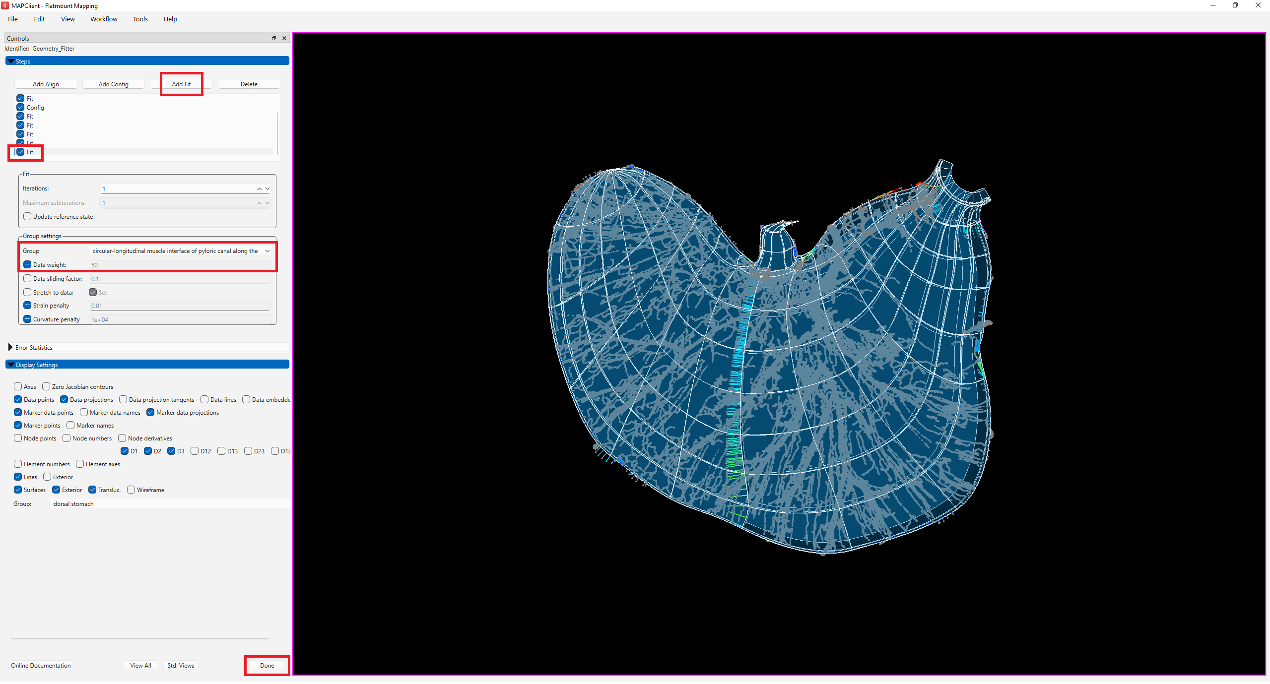
At this stage the fit looks satisfactory, to some measure (Figure 10). Add one final fit step without adjusting any parameters to ensure that the fit has reached a stable state. Additional fit steps can be added if you wish to continue to improve the fit. Multiple fit steps are always needed to converge due to non-linearity of the finite strains used in the strain penalty terms.
NoteWe are able to achieve a reasonable fit to the data with a relatively small number of steps in this example as our segmentation data is populated with sufficient points which are annotated by groups. This allowed us more control for fitting the scaffold to specific regions of the contour. If you are unable to achieve a reasonable fit to your data, consider adding more points to your segmentation data if your segmentation data is sparse. You may also wish to create more fiducial markers or groups for both your segmentation data and scaffold to facilitate fitting. Instructions on how to add fiducial markers and groups on the scaffold can be found here.
Click Done to move to the next step of the workflow.
Step 3: Embed data into the scaffold
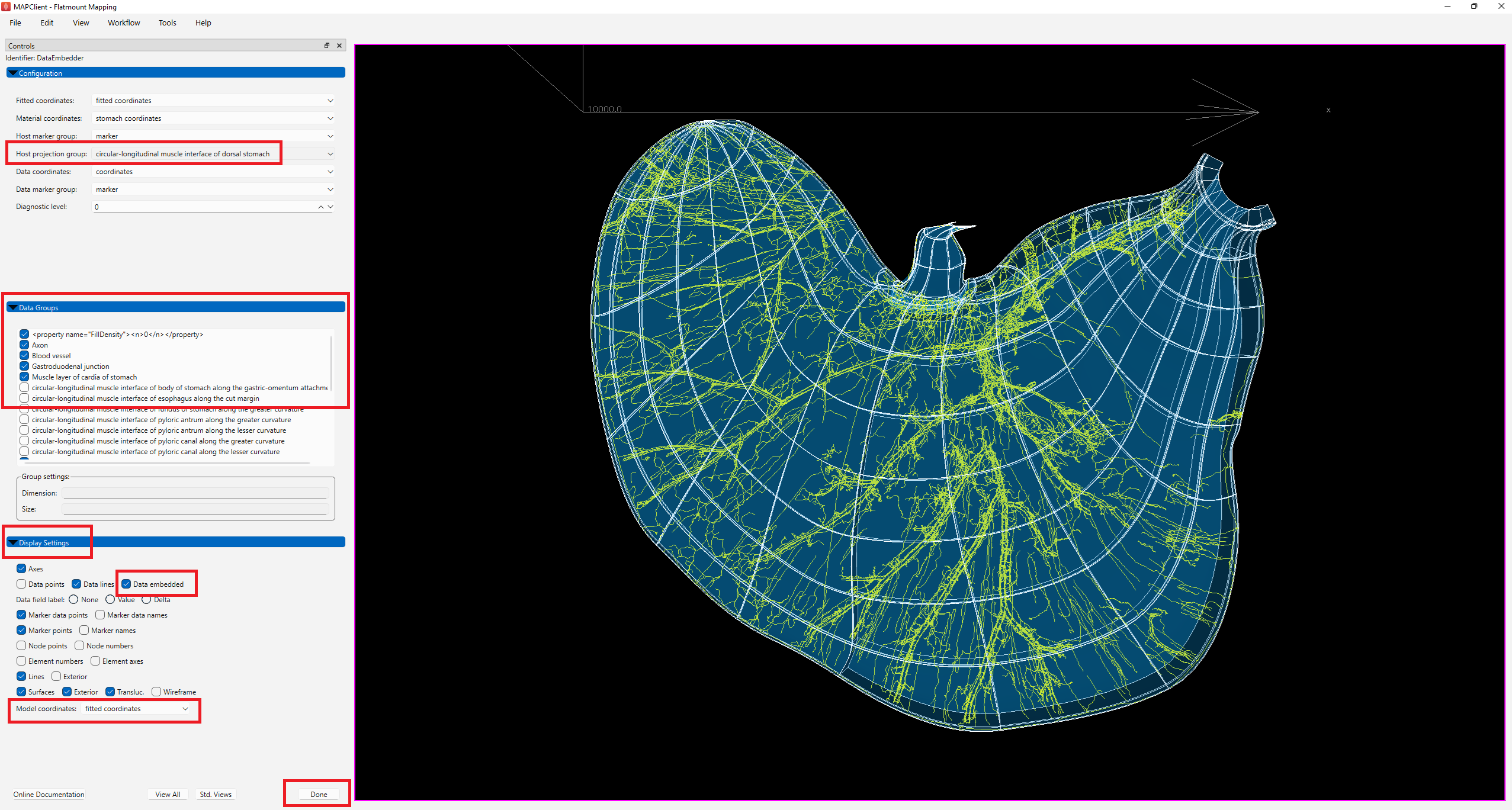
The next visual step in the workflow is the Data Embedder step. Please visit here for a more detailed explanation on how to use the Data Embedder.
Under Configuration settings, set Host projection group to circular-longitudinal muscle interface of dorsal stomach. This forces data embedding onto the surface of the selected group, so as to avoid data being embedded somewhat deeper into the volume due to fitting approximations.
The Data groups setting lists all the groups present in the data file, with a check mark beside each which shows whether the group is to be embedded. The list is automatically configured to select data groups which are present in the data but not the scaffold. User intervention may be needed to fix these initial settings to select the relevant data groups required for embedding and visualization, if necessary. In this example, we will not make any changes to the selected list.
If you wish to interrogate the embedded data in its various coordinate fields, the Display settings can be changed at any time to turn on or off graphics:
- The Model coordinates changes the coordinates shown on the scaffold, and
- Checking Data embedded engages the embedding mappings to give the value of the host's model coordinates field from the material coordinates calculated on the data.
Click Done to move on to the visualization step.
Visualize the Mapped SPARC Data on a Scaffold
Step 1: Visualize mapped data on the scaffold
In this step, we create visualization for the mapped data.
Follow steps 1 - 3 as described here, except that:
Step 1: Adding Views - It is not necessary to add a second view layout for proximal.
Step 3: Mapping - Select stomach coordinates for fields where selection is colon coordinates.
Step 4: Visualizing - Create a solid and translucent stomach material, described below, instead of the materials described in the linked documentation (Figure 12).
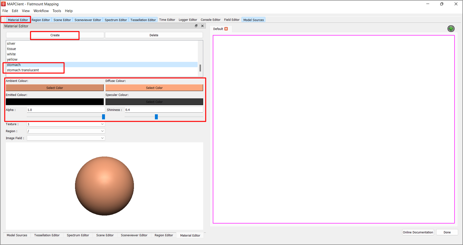
To create the materials to use in the visualization:
In the Material Editor window, click Create and rename the first temporary material as stomach. Configure the following settings and set Alpha as 1.0 and Shininess as 0.4:
| Ambient Color | Diffuse Color | Specular Color | |
|---|---|---|---|
| Hue | 20 | 20 | 0 |
| Saturation | 128 | 128 | 0 |
| Value | 211 | 252 | 56 |
Create another material and rename it to stomach translucent. This new translucent material follows the same settings as the stomach material, except that its Alpha value is 0.65.
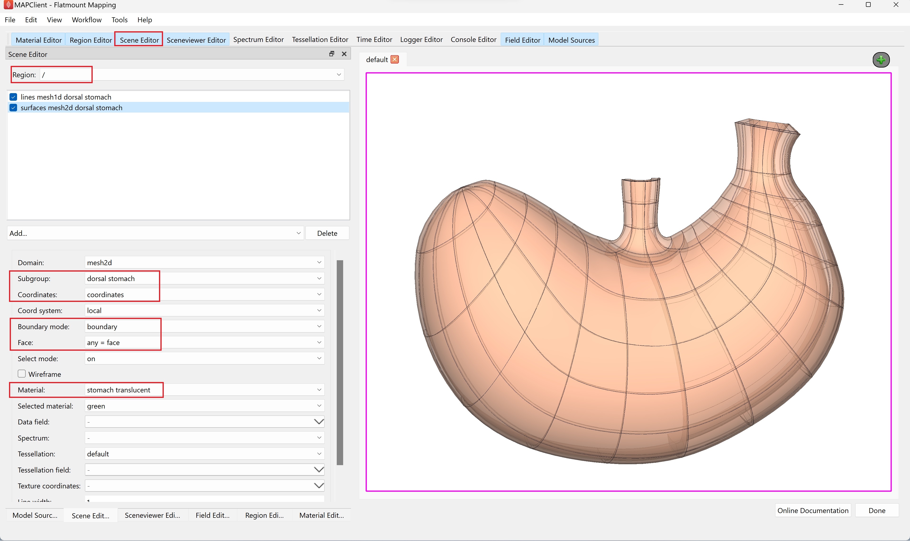
Go to the Scene Editor tab, select the Region as / and select lines from the Add graphics chooser. Under the options, set the Subgroup to dorsal stomach, Coordinates to coordinates, and Material to stomach.
Next, select surfaces from the Add graphics chooser and set the same options, except for Material, select stomach translucent instead (Figure 13). The translucency of this surface material will allow visibility of the embedded data in later steps. With the translucent material, select boundary under Boundary mode and set Face to any = face.
Next, to visualize the embedded data on the scaffold (Figure 14), select /data under Region and add lines in the graphics listing. From the options, set Subgroup as Axon, Coordinates as apply_host_coordinates, Data field as rgb, and Spectrum as rgb. To visualize the blood vessels, add lines again. This time, set Subgroup as Blood vessel, Coordinates as apply_host_coordinates, and Material as red. You may wish to increase the Line width to 2 or more to highlight the embedded blood vessels.
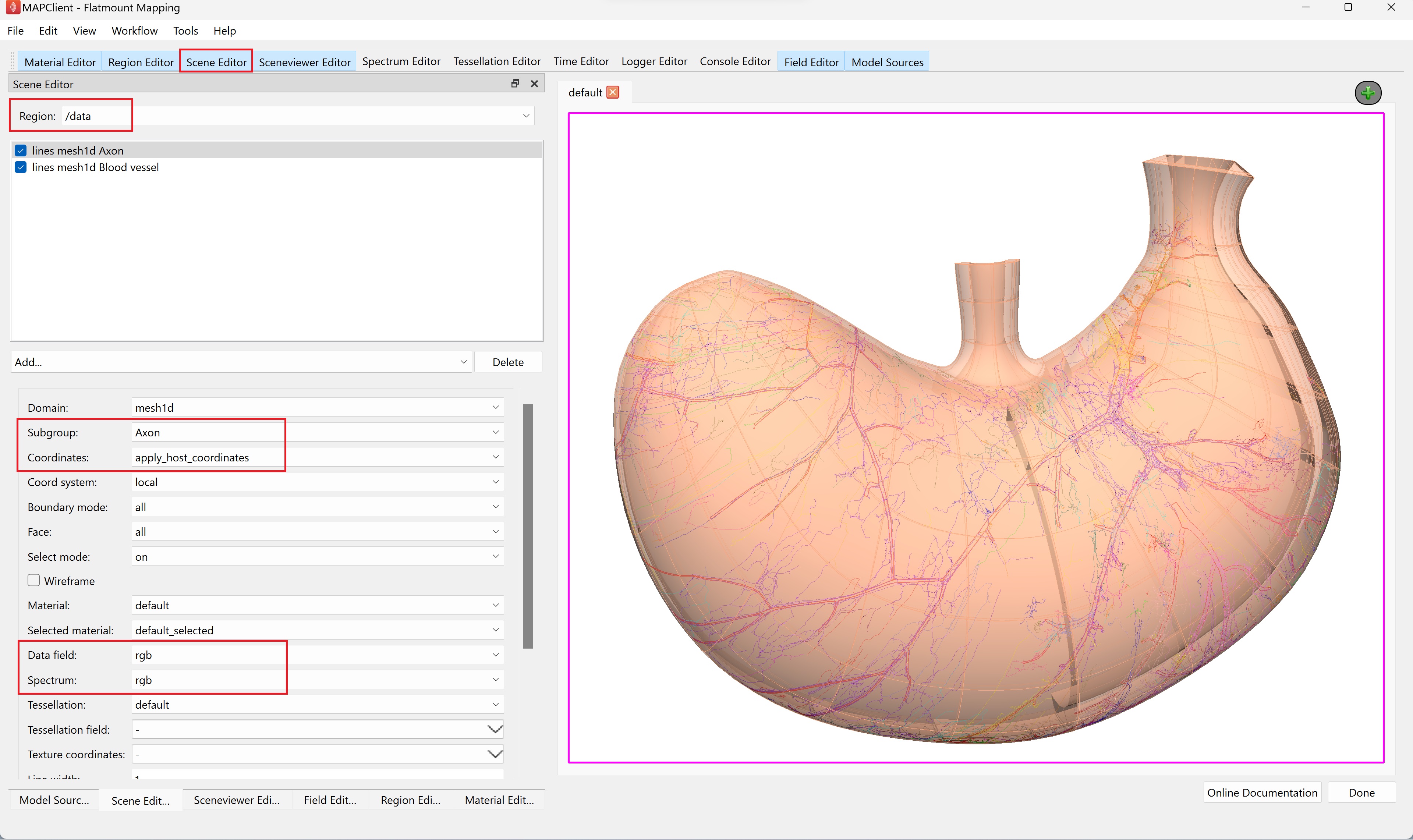
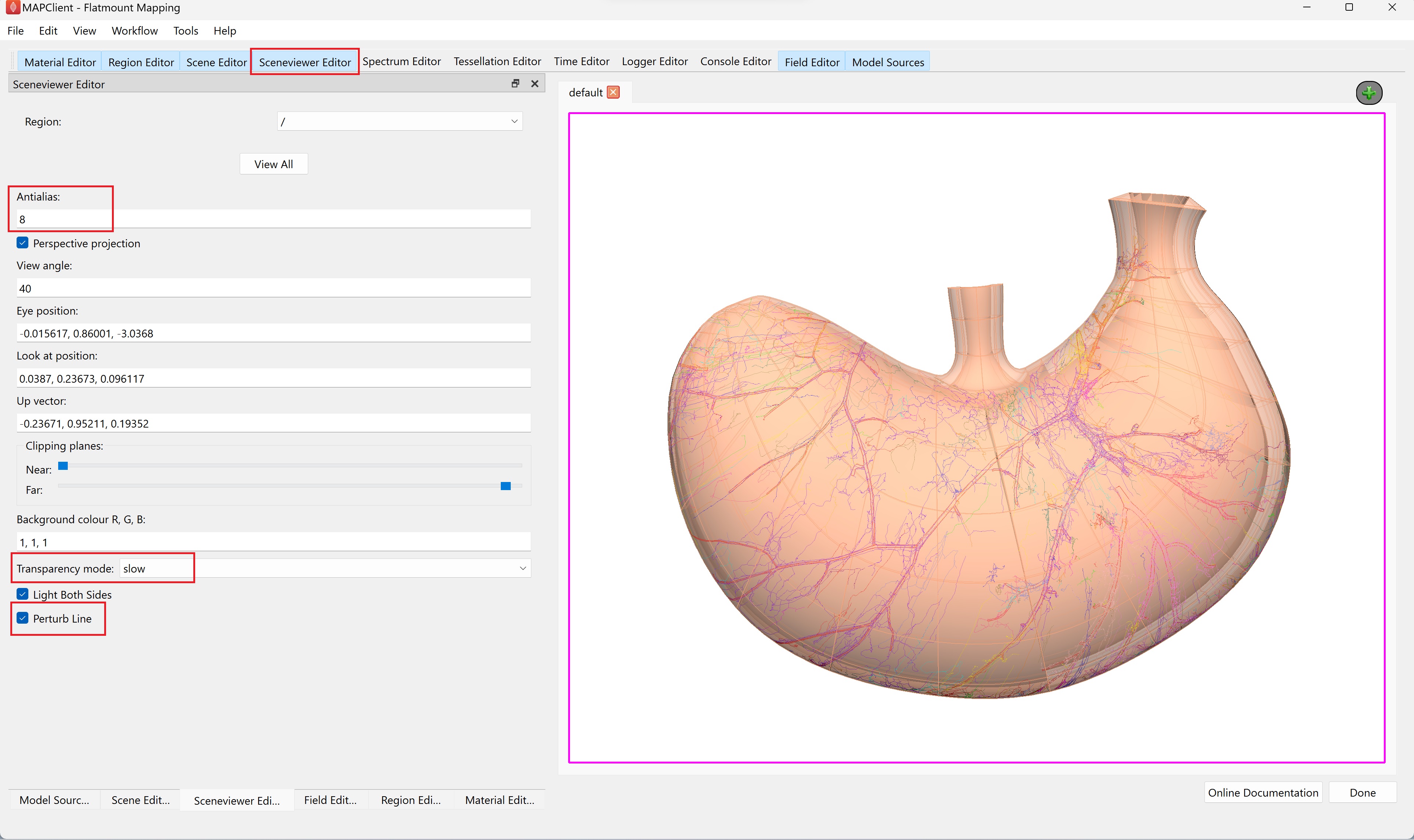
Undesirable visual artifacts are often observed when using translucent material (Figure 14). This is because we are using a simplistic calculation for which surface is in front of another. We can change this behavior by going to the Sceneviewer Editor and changing the Transparency mode to slow. To improve the smoothness of the lines, set Antialias to 8 and check the box next to Perturb Line (Figure 15).
Once you are satisfied with the visualization, click Done and the workflow will continue to generate the webGL exports and thumbnails for uploading to your SPARC dataset.
Special note
Sometimes it is advantageous to fit different data individually and visualize them on one scaffold (for example, myenteric plexus (dataEmbedder1.exf) and the axons/blood vessels (dataEmbedder2.exf) or to compare data from different samples).
To do so, open the workflow used for mapping, edit the workflow by deleting all the connections leading into the Muxer step, click on the green wheel icon on the Muxer step and change Number of inputs to 3 (Note that you can change it to any number, depending on the number of data sets you would like to combine on the scaffold).
Connect Scaffold Creator to Muxer, add two (or any number of) File Chooser steps and connect them into the Muxer (Figure 16).
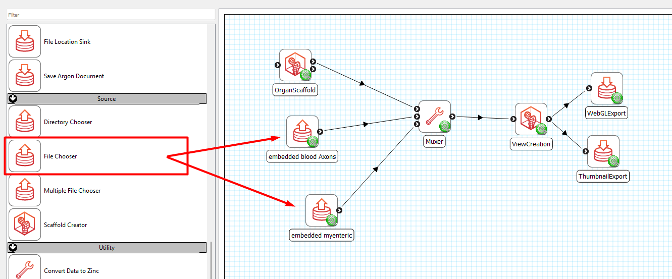
Select the dataEmbedder1.exf derived from your first workflow and dataEmbedder2.exf from your second workflow for each of the respective File Chooser. Configure where you would like to save your webGL exports and thumbnails. Save it as a new workflow and execute.
Move on to annotation or return to the main Scaffold Mapping Tools page.
Updated 11 months ago