'Model Intelligence' HyperTools on o²S²PARC
Neural Interface Safety Assessment and Model Uncertainty Quantification
Meta-Modeling is the process of establishing and exploring a (high level) model that relates input parameters of an underlying model to the associated model predictions, e.g., to understand the behavior of complex models. Especially in high-dimensional parameter spaces and for computationally demanding models, resource costs for meta-modeling can become prohibitive. Hence, intelligent algorithms combining Design-of-Experiments and Surrogate Modeling (SuMo) techniques are necessary, to enable explorations that would otherwise require thousands of time-consuming simulations. SuMos are mathematical approximations of the full model that can be evaluated much more efficiently. Corresponding 'Model Intelligence' HyperTools have recently been introduced on the o²S²PARC Platform to empower users to gain deeper insights into the impact of model parameters, to optimize designs efficiently, to quantify modeling and application uncertainties, and to make data-driven decisions with high interactivity. Forthcoming HyperTools will extend this functionality, e.g., with interactive multi-goal optimization, rare-event detection, and model-predictive control. For bioelectronic applications, where biological/inter-subject variability and design parameters interact in complex ways, meta-modeling transforms raw simulation data into actionable knowledge—revealing relationships between inputs and outcomes that might remain hidden in traditional simulation approaches. The techniques you will learn in this tutorial represent a powerful paradigm in simulation analysis, allowing you to extract maximum value from your models while strongly reducing computational burden.
Introduction
In this tutorial, you will learn how to run a Meta-Modeling pipeline on the o²S²PARC Platform in order to optimize the performance of a generic neuromodulation device—a neural interface that serves to disrupt pain signaling in the sural nerve. We will also establish confidence intervals for the optimal design parameters, accounting for the inherent variability in human tissue properties.
This tutorial demonstrates the potential of Model Intelligence HyperTools to obtain actionable insights for bioelectronic device design, balancing safety and effectivity needs.
Prerequisites
- An active o²S²PARC account: if you do not have an account on https://osparc.io/, please go to https://osparc.io/ and click on "Request Account". This will allow you to take advantage of the full o²S²PARC functionality.
Part 1: Response Surface Modeling for Implant Design Optimization
Getting Started
- Visit osparc.io and log in.
- In the Dashboard, press the “+ New” button on the top left.
- In the HyperTools section, click on the “Response Surface Modeling” option.
- A new study will open.
Note: Model Intelligence HyperTools are currently in Preview mode. For this tutorial, a pipeline has already been set up & full sampling campaigns executed, so that users can directly explore the Response Surface Modeling HyperTool’s features.
Choosing Your Function
- In the “Function Setup” step, select the “Nerve Implant Effectivity & Safety” function. It should have the defined design parameters (Inter-Electrode Spacing, Angular Width, Length, and Silicone Padding) as inputs, and the defined Quantities-of-Interest (QoIs) as outputs.
- The info button allows to visualize the underlying pipeline.
- Once all parameter ranges have been defined (for this tutorial, use the automatic pre-selection), click “Next” to move to results analysis.
- Wait until the AI model is generated. This operation might take a minute or two.
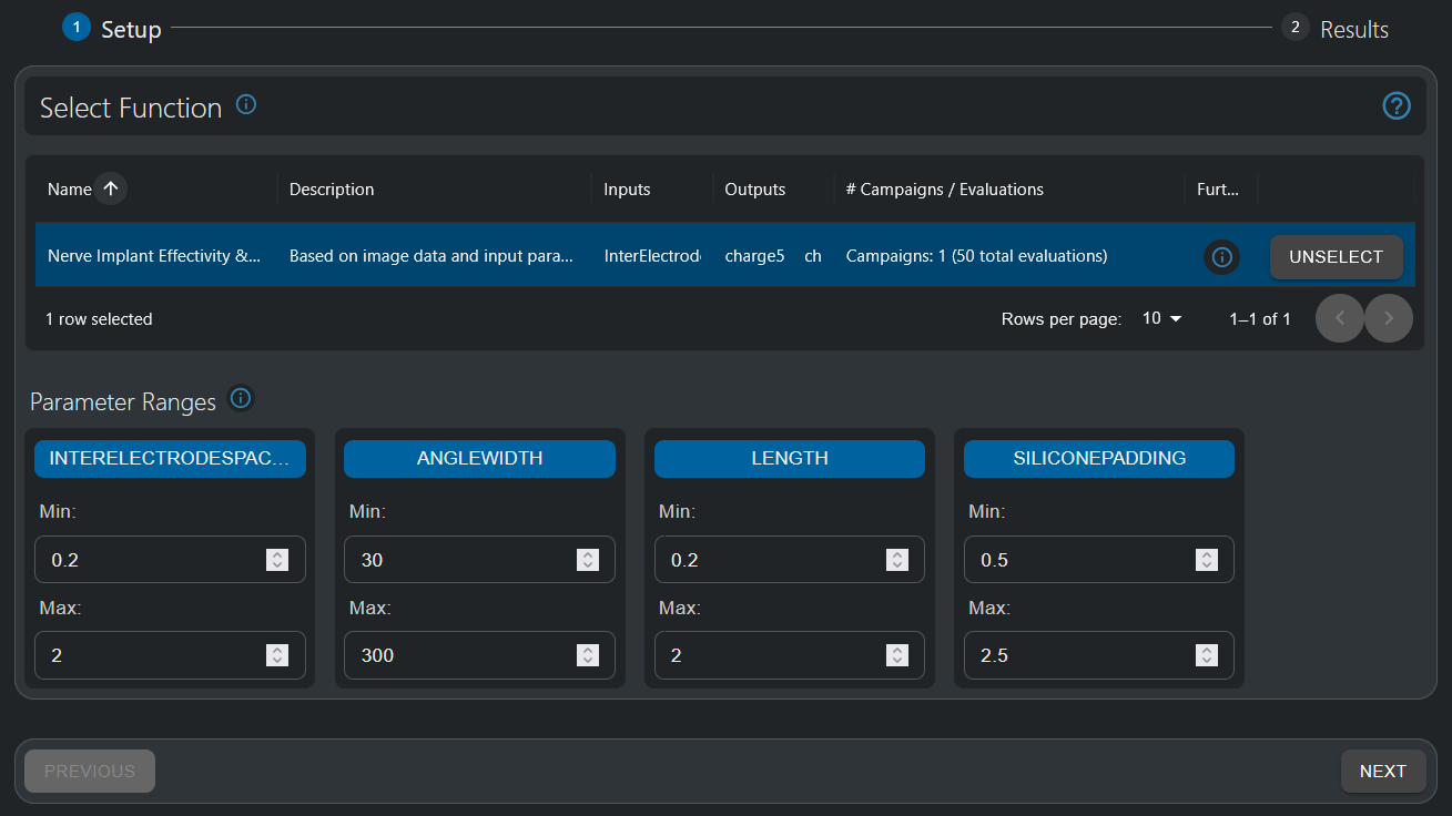
In the first step of the HyperTool, the function to be investigated is selected and parameter ranges are defined. For this tutorial, these ranges have already been pre-set.
The info button allows visualization of the underlying pipeline. In particular, the pipeline includes the following steps:
- Loading a segmented histological nerve cross-section (multifascicular).
- Generating a 2D mesh and performing a 2.5D extrusion.
- Inserting two electrodes with parameterized angular width, length, inter-electrode spacing, and extra silicone insulation padding at both ends.
- Setting up an electromagnetic (EM) simulation with parameterized conductivity for blood, epineurium, perineurium, surrounding tissue, and fascicles (longitudinal and transversal).
- Inserting and simulating fiber trajectories functionalized with electrophysiological models of neural dynamics, parameterized according to fiber diameter statistics.
- Extracting the inter-electrode impedance, dosimetric exposure quantities such as the E_IEEE/ICNIRP-averaged peak field exposure, tissue-damage-related metrics such as charge-per-phase and the Shannon criteria (of questionable relevance), as well as stimulation performance metrics such as recruitment isopercentiles (current required to recruit 5/50/95% of the fiber population).
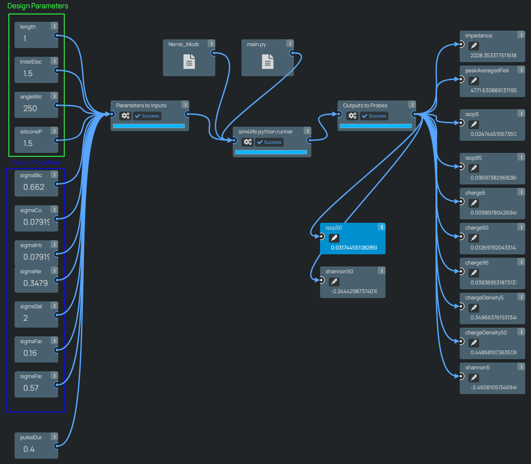
Neural interface simulation pipelines, parameterized with geometry variables and tissue properties, producing a wide range of safety and effectivity relevant predictions.
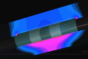
Simulated field exposure and propagating action potentials in a nerve with cuff-electrode.
Result Analysis
The 'Response Surface Modeling' HyperTool allows users to visualize the influence of one to three parameters on the selected QoI through line plots (1D), surface plots (2D), and nested isosurfaces (3D). If there are additional input parameters, their values need to be defined by the user. These values can be interactively changed using sliders, thus allowing to explore the full high-dimensional space.
Model Quality (Surrogate Model Validation)
Model Intelligence HyperTools fit a SuMo to simulated data (samples, also known as “observations”). Based on these ground-truth samples, which may take considerable computational resources to compute, a SuMo is created that approximates the input-output relationships of the full simulation pipeline. This computationally efficientSuMo can then be used to explore parameter dependencies in high-dimensional spaces, e.g., in the context of surrogate-based optimization, model-predictive control, or parameter uncertainty propagation.
Before relying on a SuMo, the user is encouraged to inspect its quality-of-fit and the results of cross-validation, which indicate, whether it is a suitable approximation of the simulation pipeline. For cross-validation, SuMos are constructed using only part of the available data and the data that was hidden during training (validation set) is compared to SuMo predictions. This procedure is performed multiple times, until all samples have been part once of the validation set. Comparing the predictions on all samples to their ground-truth (i.e., reference simulation) values provides an estimate of the accuracy of the final SuMo, which is trained using all samples.
In the first visualization of the 'Response Surface Modeling' HyperTool, a violin plot is displayed, which compares the sample values and distributions of the full-simulation observations with their cross-validation predictions. The mean and standard deviation of both the observations and the predictions’ distribution are displayed, and quantitative metrics, such as the per-sample Mean Absolute Error (MAE) and Root Mean Square Error (RMSE), are provided. Similar distributions, combined with low error metrics compared to the variance present in the data, indicates a good quality-of-fit.
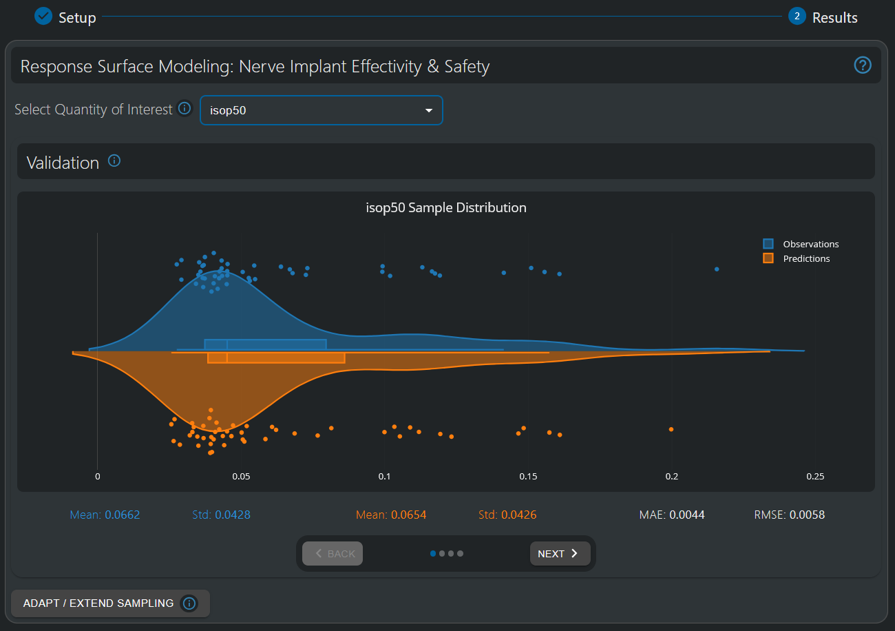
The validation window permits to assess the quality of the fitted SuMo. Violin plots compare the distribution of predicted and reference values from the cross-validation procedure. The MAE is one order of magnitude smaller than the data variance (std. deviation), i.e., the surrogate interpolation error is ~10% of the variability in the data distribution. If that compromise between SuMo quality and computational effort is inadequate, additional sampling can be run, using Design-of-Experiment techniques to select optimal configurations.
Once the SuMo quality is deemed appropriate, it is time to leverage it to gain insights into the outputs’ (QoIs) dependencies on the input parameters. For that purpose, interactive visualizations can be generated easily and efficiently through the 'Response Surface Modeling' HyperTool. Please, click the “Next” button to successively move to the 1D Curve, 2D Surface, and 3D Isosurfaces visualization tools. Note that the data (and the SuMo fitted to it) is N-dimensional (with N=4 in the first part of this tutorial), which cannot readily be visualized. However, it is possible to examine lower-dimensional “slices” or “cross-sections” of the model by fixing the values of some parameters and displaying the impact of the free parameters. It is possible to interactively change the 'fixed' values using sliders to explore their impact—or one simply modifies the assignment of parameter space dimensions to visualization axes. The provided visualization tools facilitate interactive exploration of parameter impact (sensitivity and non-linearity) and of parameter-interdependencies.
1D Curve Response
In the 1D Curves visualization tool, the X axis represents the range of values of the selected input parameter (selectable at the “Axis” dropdown below the graph), while the Y axis represents the values of the QoI of interest (selectable at the top select box).
Note: Gaussian Processes (GP) interpolation, also known as Kriging, is used for surrogate modeling. An important advantage of using GP is that it not only efficiently provides predictions for any parameter configuration, but also the associated interpolation uncertainty, which helps quantify confidence intervals. In the 1D Curve Responses, a shaded area indicates the 95% confidence interval (mean +/- twice the standard deviation for a Gaussian error distribution).
The values of the other parameters can be dynamically adapted, either by using the sliders, setting a value in the textbox, or pressing the up/down arrows in the textbox. We encourage you to explore different QoIs and to play with the interactive visualization to explore parameter dependences in different parameter “regions” of the model.
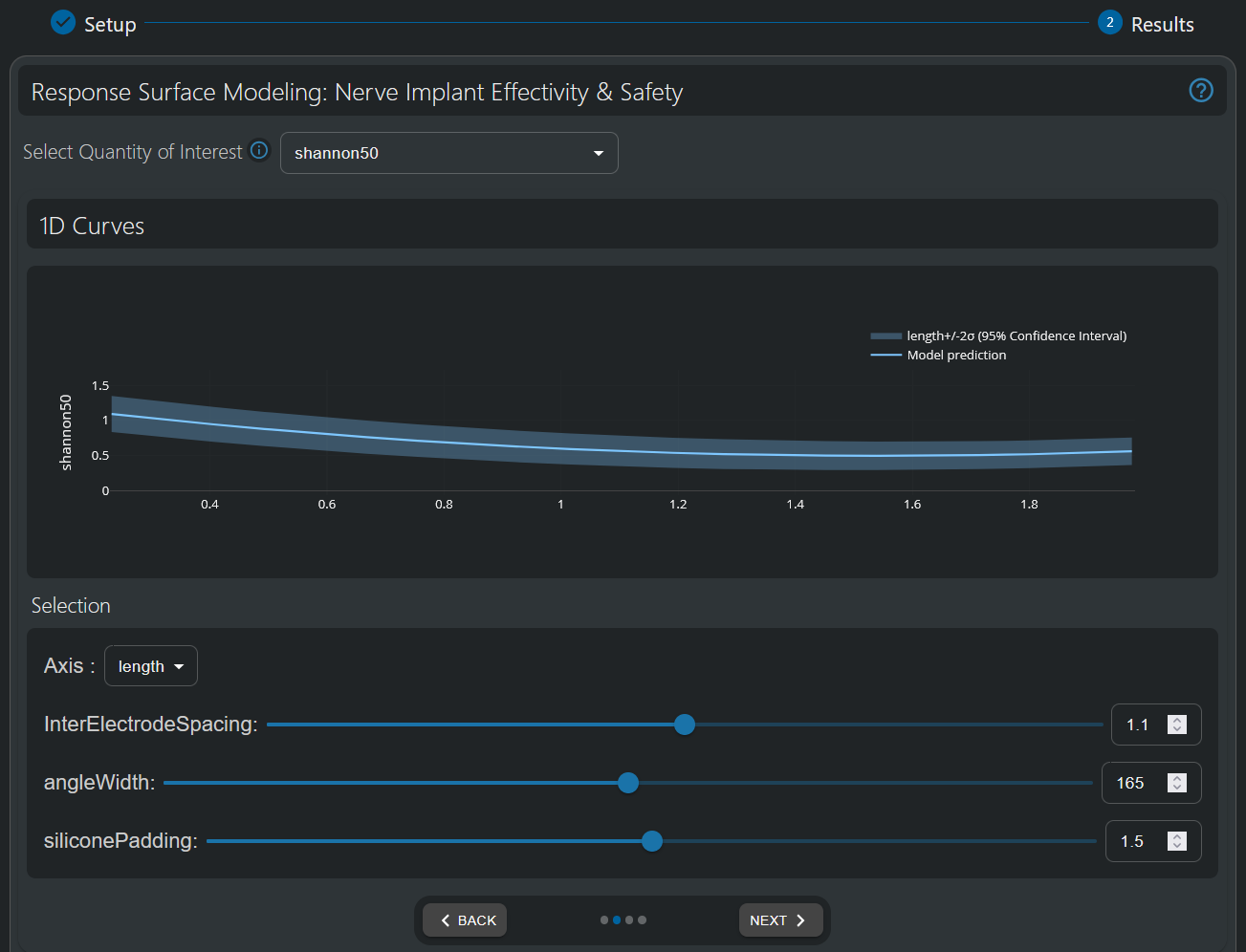
1D visualization of the electrode-length-dependence of the Shannon Criterion. The band denotes the 95% Gaussian Process interpolation confidence interval.
2D Surface Response
2D response surfaces serve to simultaneously inspect the parameter-dependence of a QoI with respect to two input parameters.
As for the 1D Curve visualization, the assignment of parameter space dimensions to plot axis can be changed using dropdowns, and the value of the remaining parameters can be interactively adapted using the sliders or textboxes.
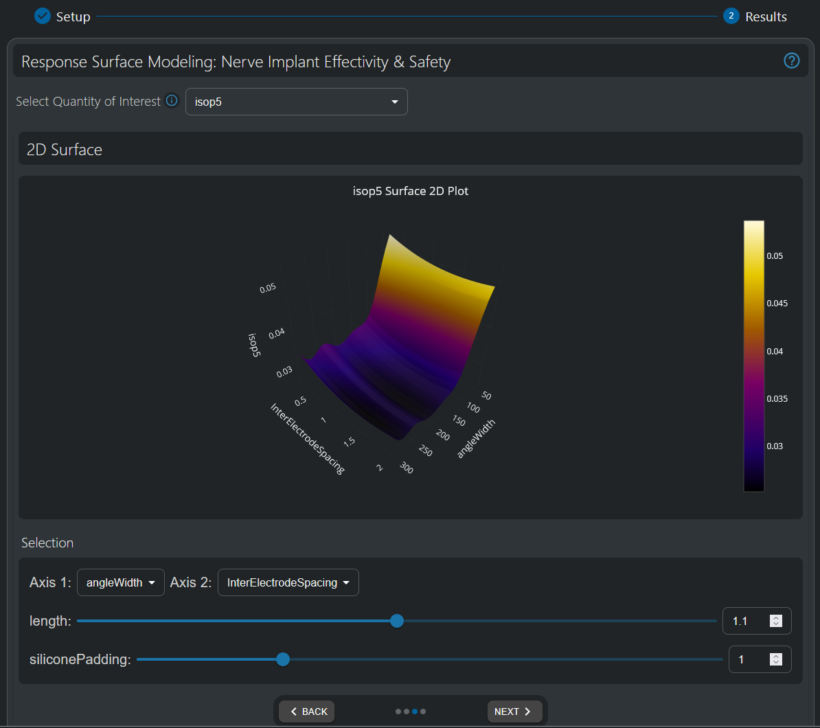
2D visualization of the 50% recruitment isopercentile threshold (i.e., the current [mA] necessary to activate 50% of the fibers in the nerve). A lower isopercentile threshold indicates easier stimulability (i.e., less current is needed to recruit the same fiber percentile) and is therefore preferrable. The electrode (angular) width is found to be a key parameter—a small width results in difficulty to recruit remote fibers. A width optimum appears to exist, though further analysis is required to ascertain, whether it is robust and general, i.e., significant compared to modeling uncertainty and nerve topology (fascicular organization) independent. Inter-Electrode Spacing has a systematic, but smaller influence—enlarging the gap reduces the 50% recruitment isopercentile threshold.
3D Iso-Surface Response
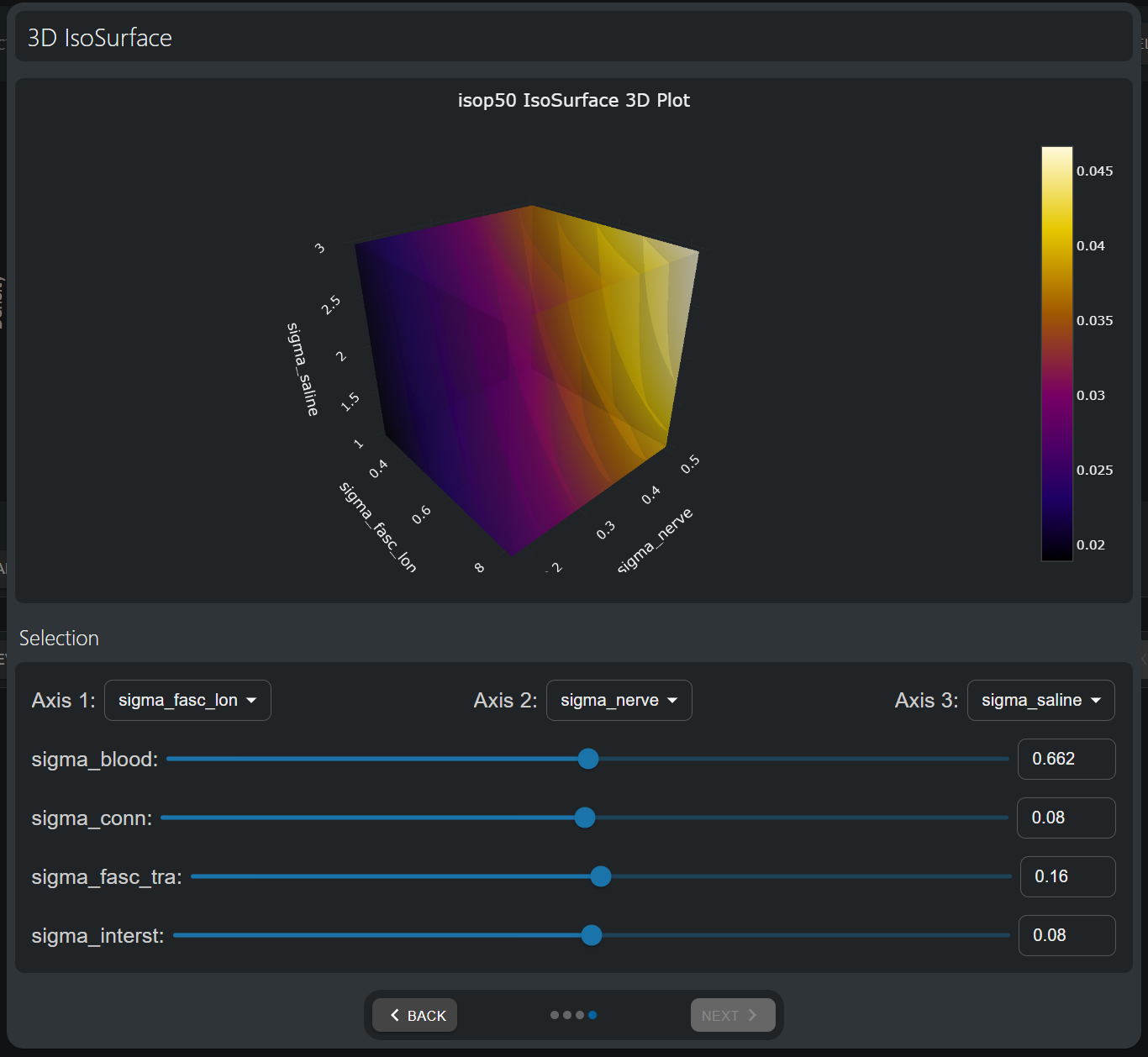
The dependence on three model parameters can be visualized through nested and color-coded iso-surfaces (i.e. the surfaces of constant QoI levels). Again, parameters of interest can be mapped to plot axes using the dropdowns below the graph, and the remaining parameters can be interactively specied using the sliders.
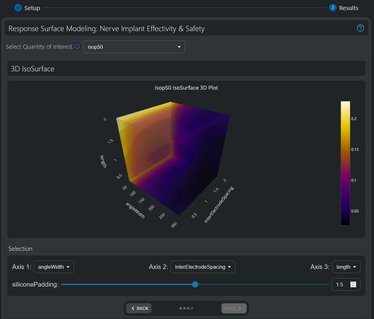
Three-dimensional visualization of the 50% isopercentile threshold (i.e. the current [mA] necessary to activate 50% of the fibers in the nerve). As already observed in the 2D visualization, higher angle widths and inter-electrode spacings both help lower stimulation thresholds. Moreover, lower electrode lengths also appears to be preferable in that respect; however, remember that it was found to adversely affect the the safety-related Shannon Criterion in the 1D plot analysis.
Selecting a Design
Using these visualizations qualitative and quantitative insights can be gained. We use them to define design parameters of the sural nerve implant stimulator, which strike a compromise between effectivity (isopercentile threshold current at 50% fiber recruitment, isop50) and safety (Shannon Criteria at the same current level, shannon50).
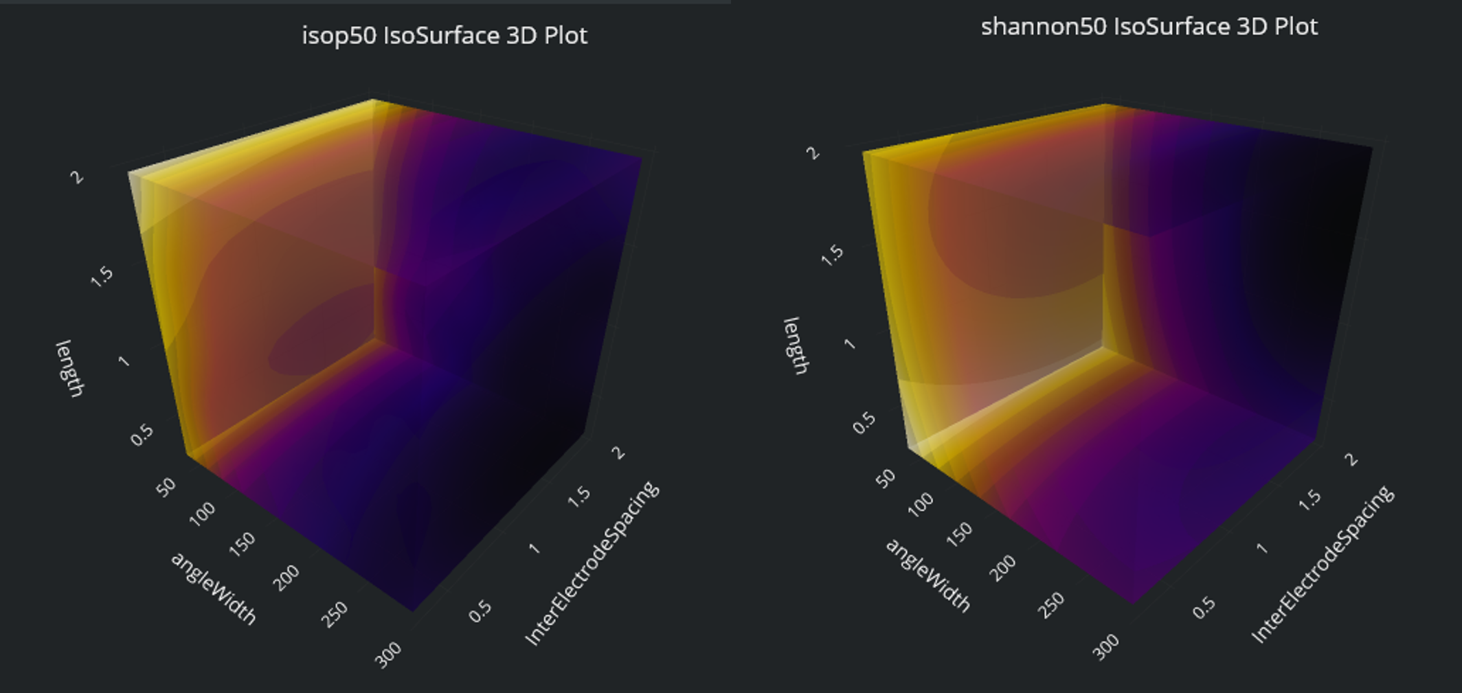
3D visualizations of the two main quantities of interest, 50% isopercentile threshold (i.e. current [mA] necessary to activate 50% of the fibers in the nerve) and Shannon Criteria at that current level, which should both be minimized for enhanced effectivity and safety. While both metrics seem to benefit from large angular widths and inter-electrode spacing, smaller length benefits effectivity but harms safety, such that an intermediate value isas a compromise.
The insights gained on the three-dimensional visualizations can be further explored through one-dimensional cross-sections, which also provides estimates of uncertainty. The figure shows dependence on the angle width and length parameters (which play the largest roles) on both 50% isopercentile current and Shannon Criteria. As seen in the three-dimensional visualizations, while both efficiency and safety benefit from wider angle width, an intermediate length value appears to offer a good compromise.
Based on the above visual exploration, the following design parameters were chosen as optimal:
- Angular Width : 250º
- Inter-Electrode Spacing: 1.5mm
- Length: 1mm
- Silicone Padding: 1.5mm
This configuration should produce 50% fiber recruitment at a current 0.03mA, with an associated Shannon Criterion value around -2.2 (well below and on the safe side of the typically employed threshold of +1.85).
Comparison of the reference model evaluation ('Observations') distribution and the cross validation estimations ('Predictions') for two main outputs of interest (50% isopercentile current and Shannon Criteria at that current level). The two distributions are in close agreement, supporting the quality of the SuMo.
Validation of Design Parameters through Full Simulation Pipeline
In order to confirm that the design parameters identified as optimal based using the Response Surface Modeling HyperTool are indeed well predicted by the underlying SuMo, the tool allows to explicitly simulate a specific parameter configuration of interest. For that, we enter the identified design parameters under Adapt / Extend Sampling -> Create new sampling campaign -> Test run. A new simulation is setup, configured in accordance with the specified configuration, and opened in a new tab for execution and extended analysis.
Indeed, running the full pipeline for the selected parameter configurations confirms a 50% recruitment current of 0.032mA and an associated Shannon Criterion of -2.24.
Implant Design Optimization—Conclusion
In this tutorial, we have explored how Response Surface Modeling can transform complex bioelectronic simulations into actionable design insights. Through that Model Intelligence HyperTool, we were able to:
- analyze parameter dependencies across a multidimensional design space without running thousands of simulations;
- visualize critical relationships between design parameters (electrode dimensions, spacing, insulation) and performance metrics;
- balance competing efficacy (lower isopercentile threshold) and safety (lower Shannon criterion) objectives;
- Make data-driven design decisions that would be computationally expensive using traditional parameter sweeping.
The analysis revealed that:
- wider angle coverage (around 250°) significantly improves nerve fiber recruitment;
- larger inter-electrode spacing (1.5mm) reduces stimulation thresholds;
- for electrode length, a tradeoff between efficacy and safety considerations is necessary, and an intermediate length is judged to be optimal;
- increased silicone padding (1.5mm) contributes to an optimal design (including mechanical considerations could change that).
The performance predicted by the SuMo for the chosen configuration was validated through full simulation, confirming that our optimized design achieves the desired 50% isopercentile current under 0.05mA, while maintaining a Shannon Criterion below -2.0—well within safe limits.
This tutorial demonstrates how Model Intelligence tools can strongly facilitate and accelerate the bioelectronic device design process, reducing computational overhead while providing deeper insights into complex parameter relationships. They transform raw data into actionable knowledge that can directly inform better and safer bioelectronic interventions.
Part 2: Uncertainty Analysis and Confidence Interval Quantification
The second part of this tutorial demonstrates the use of a second Model Intelligence Hypertool to establish confidence intervals with regard to tissue property uncertainties for the identified optimal design parameters. Tissue properties are uncertain, both as a result of inter- and intra-subject variability, as well as the challenge of measuring them.
The 'Uncertainty Quantification' HyperTool provides an easy-to-use framework for propagating uncertainty about underlying parameters through a complex and non-linear model, revealing insights into the resulting probability maps for the predicted QoIs—a key requirement when generating in silico evidence for regulatory submissions.
Getting Started
- Visit osparc.io and log in.
- In the Dashboard, press the “+ New” button on the top left.
- In the HyperTools section, select the “Uncertainty Quantification” option.
- A new study will open.
Choosing your function
- In the Function Setup step, select the Tissue Conductivity Uncertainty - Nerve Implant Effectivity & Safety function.
- It has tissue conductivities (typically denoted with a sigma) as inputs, and the QoIs already encountered in the first tutorial part as outputs. The info button permits to visualize the underlying pipeline.
- For this tutorial, parameter probability distributions have already been defined. They are all assumed to be Gaussian with means set according to reference values from literature (IT’IS Low Frequency Tissue Database) and standard deviation that were uniformly assumed to be 20% of the mean value.
- Click “Next” to move to the result analysis step.
- Wait until the AI model is generated. This might take a few minutes.
After a function to be analyzed has been selected in the 'Uncertainty Quantification' HyperTool, parameter probability distributions (constant, uniform, normal) can be defined. For this tutorial, normal (Gaussian) distributions are used, with mean values set according to literature IT’IS Low Frequency Tissue Database and standard deviations assumed to be 20% thereof.
Result Analysis
The 'Uncertainty Quantification' HyperTool allows users to quantitatively assess output variability as a result of input parameter probability distributions, and to establish rigorous confidence intervals for the modelled efficiency and safety metrics. This is a critical requirement, e.g., for regulatory-grade modeling and for ensuring that a device design is robust and suitable across the relevant inter-subject variability of a target population.
Sensitivity analyses often study the impact of individual variables on a quantity-of-interest in isolation—investigating the interplay between multiple uncertain parameters quickly becomes computationally expensive as a result of the curse of dimensionality (the parameter space grows exponentially with the number of parameter dimensions; for example: spanning a grid with only 3 samples per axis for the six parameters in this tutorial would already result in over 700 configurations. The 'Uncertainty Quantification' HyperTool uses an alternative approach:
- A low density Lating Hypercube Sampling of the parameter space is generated (50 samples in this tutorial) and the corresponding configurations are simulated
- A Gaussian Process SuMo is fitted to the simulated data (observations).
- This SuMo can be used to efficiently evaluate a high-density sampling of the input parameter space (Number of UQ Samples, 10.000 by default) according to their statistical distributions previously specified by the user.
- Statistical descriptors and a visualizing histogram of all propagated samples are computed for the selected QoI, accounting for model non-linearities and the complex interplays between parameters.
This methodology provides a superior uncertainty computation than classic approaches that combine (e.g., using root-sum-square) uncertainties contributions obtained through sensitivity analysis of individual parameters. Furthermore, by repeating this procedure 50-times with stochastically varying parameter space sampling and accounting for the interpolation uncertainty of the Gaussian Process SuMo, the uncertainty of the probability distribution can also be quantified ('uncertainty of uncertainty'). It is visualized by error bars in the Uncertainty Propagation Histogram. Large error bars suggest that either more configurations must be simulated for the SuMo construction (reduce the interpolation uncertainty), or that the parameter space sampling using the SuMo must be increased.
Probability distribution of isop50, the current required to recruit 50% of the fibers. An important variability (>10% standard deviation) is apparent.
The histogram for isop50 (the current required to recruit 50% of the fibers) shows an important width: The standard deviation is 0.004mA, compared with an expectation value of 0.032mA (i.e., a >10% variability resulting from 20% uncertainty in the underlying tissue conductivities). Analysis of the SuMo shows that the dominant factors are the conductivities of nerve tissue and the surrounding medium ('saline'), as well as the longitudinal part of the fascicular conductivity.
The variability of isop50, the current required to recruit 50% of the fibers, primarily results from the uncertainty associated with the conductivities of nerve tissue and the surrounding medium ('saline'), as well as the longitudinal part of the fascicular conductivity.
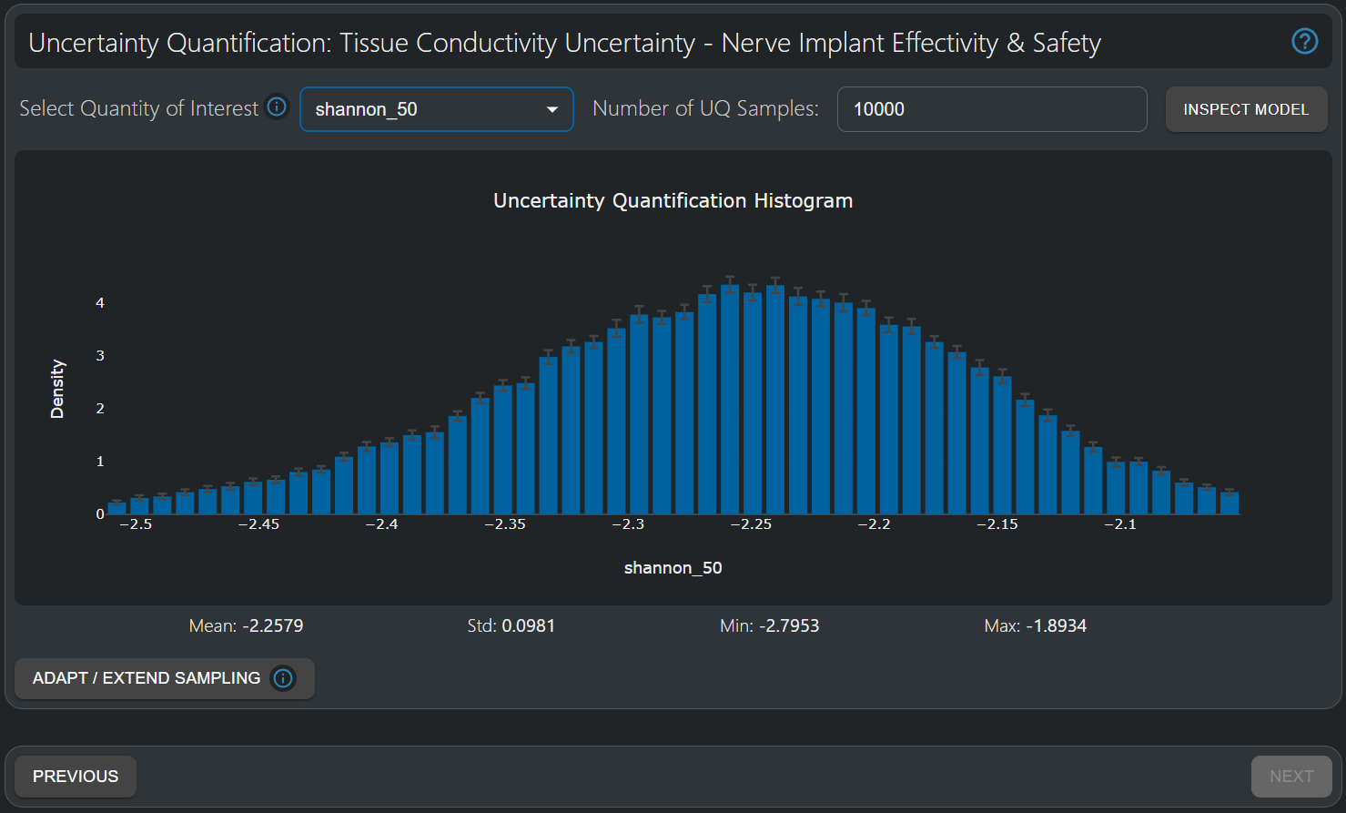
The Uncertainty Quantification Histogram provides a comprehensive statistical description of the output quantity of interest, accounting for non-linear parameter dependencies and parameter interplay. Here, the distribution of the values of the Shannon Criteria at 50% current threshold isopercentile (i.e. the current [mA] value at which 50% of the fibers in the nerve have been activated) is shown—a quantity frequently reported in the context of stimulator implant safety with regard to electrochemical effects. The mean (-2.23) is close the value predicted for the optimal design parameters (-2.24) in the previous tutorial. The distribution is approximately Gaussian with a narrow standard deviation (0.066) , despite the 20% uncertainty associated with the parameterized tissue conductivity distributions. Hence, it is unlikely that the Shannon criterion approaches the +1.85 threshold.
Interestingly, the tissue conductivity uncertainty has only a small impact on the Shannon safety criterion (+/-0.1), presumably because of its logarithmic nature. The dominant parameters are the longitudinal fascicular and the nerve tissue conductivities.
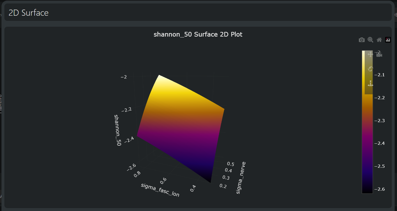
Sensitivity of the Shannon criterion at a level required to recruit 50% of fibers to the dominant tissue parameters: the nerve conductivity and the longitudinal fascicular conductivity.
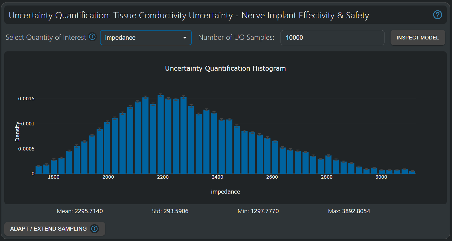
The tissue impedance has a higher relative standard deviation than the 50% recruitment isopercentile and is significantly affected by all parameterized tissue conductivities in the model.
Validate Model Quality
The Uncertainty Quantification Histogram relies on a SuMo fitted to the sampled data (observations), and the accuracy of the predicted histogram relies on a good quality-of-fit of this SuMo.
The Inspect Model button on the top-right corner enables users to assess the model’s quality-of-fit through cross-validation. Additionally, 1D / 2D / 3D visualizations of the parameter-impact on QoIs can be utilized to gain further insights key parameters that have an important impact on the total uncertainty. For additional explanations, see the first part of this tutorial.
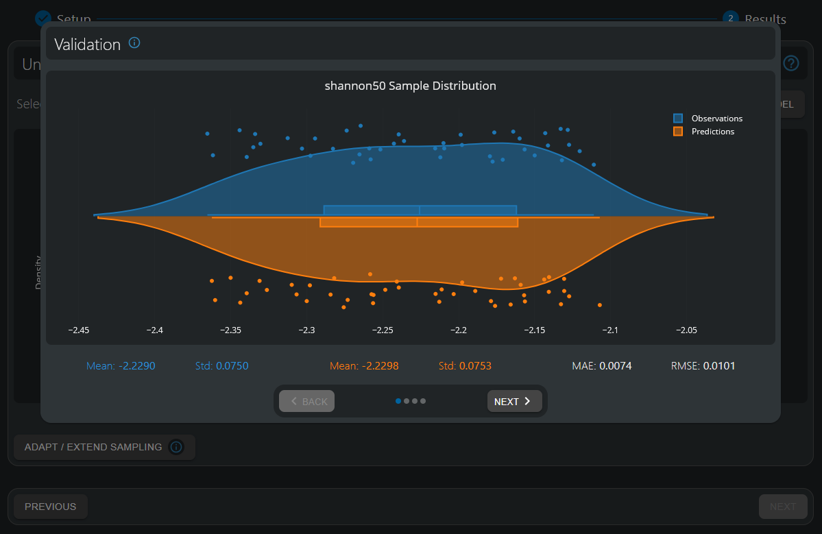
The distribution of simulated data (observations) and surrogate predictions are highly aligned, with a per-sample mean absolute error (MAE) of 0.0074—approximately 10% of the overall standard deviation in the data (0.075)—indicating a sufficient quality-of-fit.
Uncertainty Quantification—Conclusion
In this part of the tutorial, we have demonstrated for a bioelectronic implant design example application, how the 'Uncertainty Quantification' HyperTool provides an intuitive and powerful framework for assessing the uncertainty of predicted QoIs as a result of model parameter uncertainty. By efficiently propagating input uncertainties through a SuMo, we established the associated confidence intervals for safety and efficacy metrics—a critical requirement for in silico regulatory evidence and the preparation of clinical translation.
Key takeaways from this tutorial:
- With just 50 simulation samples, we could characterize the statistical distribution of output metrics in a seven dimensional parameter space, which would require thousands of simulations using grid exploration.
- Cross-validation confirmed the suitability of the SuMo, supporting its application for uncertainty propagation.
- The presented methodology properly accounts for the complex interplay between biological variability / measurement uncertainty and design parameters, handling non-linearities and parameter inter-dependencies.
The 'Uncertainty Quantification' HyperTool permits to transition from deterministic to probabilistic design, allowing engineers to efficiently quantify and communicate the statistical reliability of their designs—a capability increasingly demanded by regulatory bodies and essential for successful clinical translation of bioelectronic therapies.
Conclusion
This tutorial demonstrates the value of o²S²PARC's Model Intelligence Hypertools. They readily enable users to obtain actionable insights for bioelectronic device design, enabling a choice of parameters that optimally balances effectivity and safety metrics, and to establish associated confidence intervals—a critical requirement for regulatory submission and clinical translation. Through Design-of-Experiments and surrogate-modeling techniques, the number of required simulations can be dramatically minimized.
Note: Model Intelligence HyperTools are currently in Preview mode. We will be happy to provide you with full-featured access upon request to our support channels. Happy meta-modeling!
Updated about 1 year ago