Running a MetaModeling Pipeline On o²S²PARC
In this tutorial you will learn how to run a Meta-Modeling pipeline on the o²S²PARC Platform, in order to evaluate the performance of a neuromodulation device with the clinical goal of preventing chronic migraine episodes, and optimizing its performance with the simultaneous goals (and often opposed) of maximizing stimulation performance and minimizing energy consumption.
Prerequisites
- An active o²S²PARC account: if you don't have an account on o²S²PARC, please go to https://osparc.io/ and click on "Request Account". This will allow you to take advantage of the full o²S²PARC functionality.
- Basic knowledge of the JupyterLab environment: if you wish to only run the code and visualize the results, you really need only the basics. See here for an introduction.
Introduction
Stimulation of sub-cutaneous nerves has been found to ameliorate symptoms of chronic migraine. A human model from IT'IS Virtual Population was extended with sub-cutaneous cranial nerves and an implant was inserted. Exposure from an electrical stimulus was simulated using Sim4Life.
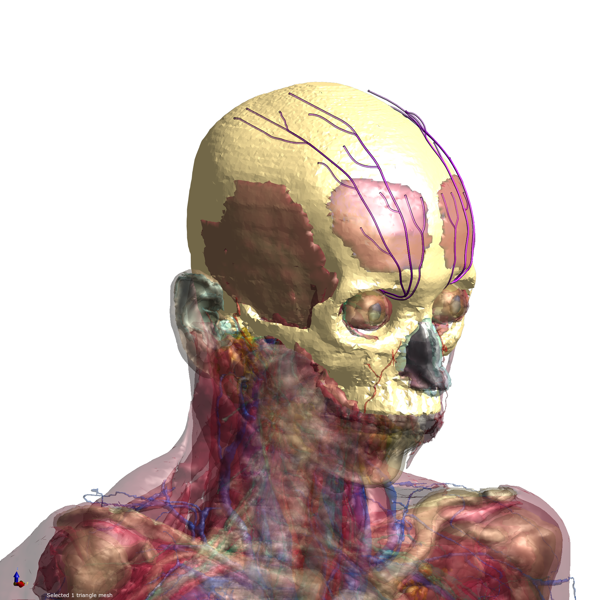
Figure 1: Virtual Population model inside Sim4Life.
Based on this exposure data, stimulation effects on neural fibers inside the sub-cutaneous nerves can be computed through the Generalized Activating Function, an accurate approximation of NEURON simulations which provides a very considerable speed-up without compromising accuracy.
This tutorial is divided in three parts. Parts 1 and 2 explain and build up knowledge about the MetaModeling framework and provide useful know-how; Part 3 showcases a realistic use case for MetaModeling for peripheral nerve stimulation.
Part 1 - Evaluate pre-defined sample points illustrates the basics of the Meta-Modeling framework: how to create samples (a pre-defined pulse shape at different amplitudes), create a Dakota input file, and perform multiple evaluations of these inputs through the ParallelRunner service.
Part 2 - LHS Sampling of the input space expands the previous part by illustrating how to generate samples in a randomized way using the Latin Hypercube algorithm within Dakota, and visualizing both inputs and outputs.
Part 3 - Pulse Shape Optimization (Advanced) illustrates a complex, real-life use-case: optimization of a pulse shape for a neurostimulation device. A genetic algorithm is used to automatically generate pulse shapes which then are evaluated through the Runner. Furthermore, a surrogate model is built and iteratively refined to further speed-up and improve convergence.
Goals
This tutorial aims to show how the o²S²PARC's Meta-Modeling framework can be utilized to analyze a realistic clinical model through multiple evaluations using the Parallel Runner Service. This feature can be exploited for various meta-modeling workflows: optimization, uncertainty quantification, surrogate-model building... An integrated Dakota Service is provided, which combines ease-of-use and flexibility, and also provides a base for advanced users to set up their own workflows.
Getting Started
Before starting, be sure to be logged in o²S²PARC (by visitinghttps://osparc.io/). If you are not logged in, you will see an error message prompting you to log in.
Once you are logged in, you can clone the MetaModeling Tutorial template:
- Go to https://osparc.io/ and click on the "Templates" tab
- Type "MetaModeling Tutorial" in the search bar
- Click on the "MetaModeling Tutorial" template
- Click on "Open" in the Template Details window
In this way, a copy of the template as a new o²S²PARC Study in your Workspace. This is your own copy, so feel free to make changes and try edit the parameters in this tutorial - you can always come back to this step and create a new copy from the public template.
Understanding the o²S²PARC's Meta-Modeling study structure
](https://files.readme.io/413e4ea5456e6678911fe6f8b827d5f30a90e059059c4881da4e8d37ad912747-image.png)
Figure 3: Study view of the Tutorial in o²S²PARC
Studies that use o²S²PARC's Meta-Modeling framework typically follow this hour-glass structure:
- JupyterLab: interactive service which allows the user to define the parameters to be evaluated, as well as retrieve and analyze results.
- ParallelRunner: receives a list of parameter sets to be evaluated, and controls job creation, execution and result retrieval.
- DakotaService: transforms human-readable configuration files into samples to be run, and can perform additional meta-modeling tasks such as sampling, model building, and iterative optimization.
NB: While the DakotaService is not strictly necessary (it would be possible to directly provide parameter sets from the JupyterLab to the ParallelRunner), Dakota's flexibility and the Service's purpose-built mapping interface towards the ParallelRunner make it the most convenient option, even for simple parameter evaluations.
Additionally, two configuration JSON files are provided:
- Dakota Settings (optional): allows to adjust various options, such as restart-ability after errors in the Dakota workflow.
- Parallel Runner Settings (necessary): it allows to provide the ID of the template to be executed (see the Advanced section at the end of the tutorial for more details on setting up this template) and other options such as number of parallel workers or optionally define a job timeout time.
To start running the tutorial, select the JupyterLab - Tutorial service, choose the interactive view (also available by clicking twice on the service box) and open the Tutorial.ipynb notebook. Please execute the code cells sequentially, after reading the corresponding part of the tutorial. Feel free to play with the code and parameters - it is always possible to create a fresh copy of the Tutorial!
Setup
The first cells of the notebook import necessary libraries and oSPARC libraries, define the input and output paths of the service, and start the communication between the JupyterLab service and the DakotaService via handshake. Executing the handshake might take up to a minute.
Furthermore, some hard-coded parameters must be provided. These are copied from the Runner template (see the Advanced section at the end of this tutorial for more details) and establish the number of variables that the template accepts. Please, do not modify these values.
Part 1 - Evaluate pre-defined sample points
This first part of the tutorial will exemplify how the Meta-Modeling framework can be used to evaluate an arbitrary number of input configurations in parallel, substituting an otherwise manual, tedious and error-prone task, especially for complex pipelines with long execution times.
Generation of the input file
A biphasic stimulation pulse of 0.3ms phase duration will be evaluated for a range of amplitudes, thus quantifying the relationship between stimulus amplitude and nerve activation for a fixed pulse shape.
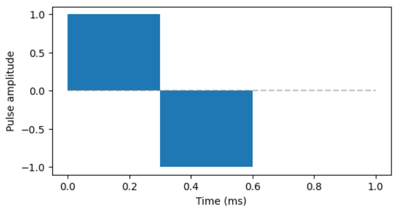
Figure 4: Biphasic pulse to be evaluated.
A file containing all pre-defined input configurations is generated (BiphasicPulses.csv) and can be inspected by the user. Alternative phase duration and amplitude ranges could also be explored by the user. Please note - valid pulse phase duration are 0.1 - 0.4ms, and any real (float) value as amplitude is valid. A negative value will simply invert the pulse (e.g. cathodic phase first, anodic after).
The Dakota configuration file
Now that the input file is generated (and copied to the output folder), it is time to create a Dakota configuration file to execute it. Meanwhile Dakota is not strictly necessary to execute multiple evaluations with the ParallelRunner, its power and flexibility, as well as human-readable interface, make it the easiest option. Furthermore, this example allows to provide an introductory example to Dakota input files, over which subsequent parts of this tutorial will build. Please execute the cell containing the create_dakota_conf_eval function and inspect the resulting configuration file:
environment
    tabular_data
        tabular_data_file = 'results_eval.dat'

    method
        id_method "EVALUATION"
        model_pointer 'EVALUATOR'

        list_parameter_study
            import_points_file
                './BiphasicPulse.csv'
                custom_annotated header

    model
        id_model = 'EVALUATOR'
        single
            interface_pointer = 'INTERFACE'
            variables_pointer = 'VARIABLES'
            responses_pointer = 'RESPONSES'

    interface,
        id_interface = 'INTERFACE'
        batch
        python
            analysis_drivers
                'model'

    variables
        continuous_design = 9
        id_variables = 'VARIABLES'
            descriptors 'p1' 'p2' 'p3' 'p4' 'p5' 'p6' 'p7' 'p8' 'p9'

    responses
        id_responses = 'RESPONSES'
        descriptors '1-activation' 'energy' 'maxamp'
        objective_functions = 3
        no_gradients
        no_hessians
The Dakota configuration file has the following key elements:
- Method: top-level element - in this case, a list of parameters to be evaluated, and references the input file we have previously generated
- Model to be evaluated by the method. This is in principle any black-box that is composed by the following elements:
- the variables - these are the inputs to our evaluation pipeline, and the input descriptors must match the input keys in the underlying pipeline.
- the interface points to the evaluation pipeline itself. The settings of the interface in this tutorial are tailored to the ParallelRunner and should not be modified.
- the responses - these are the outputs of our evaluation pipeline. These must match the keys in the output dictionary / JSON file of the underlying pipeline.
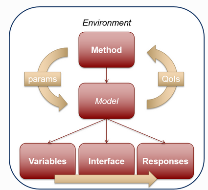
Figure 5: Diagram of the different elements of a Dakota workflow.
Executing Dakota
Once the Dakota configuration file (named as dakota.in) is copied to the output folder of the JupyterLab service and transferred to the DakotaService, the latter will start executing the provided configuration file through Dakota.
NB: any additional files (e.g. the input file BiphasicPulses.csv) must be provided in the output folder PRIOR to writing / copying the dakota.in file which will trigger the execution of the pipeline.
While Dakota is executing, nothing will display in the JupyterLab. Therefore, head to the logs (third icon in the top center menu of oSPARC) to see the DakotaService printouts, and then, to the ParallelRunner interactive window to see the execution status of your jobs (ToDo / Running / Done / Failed):
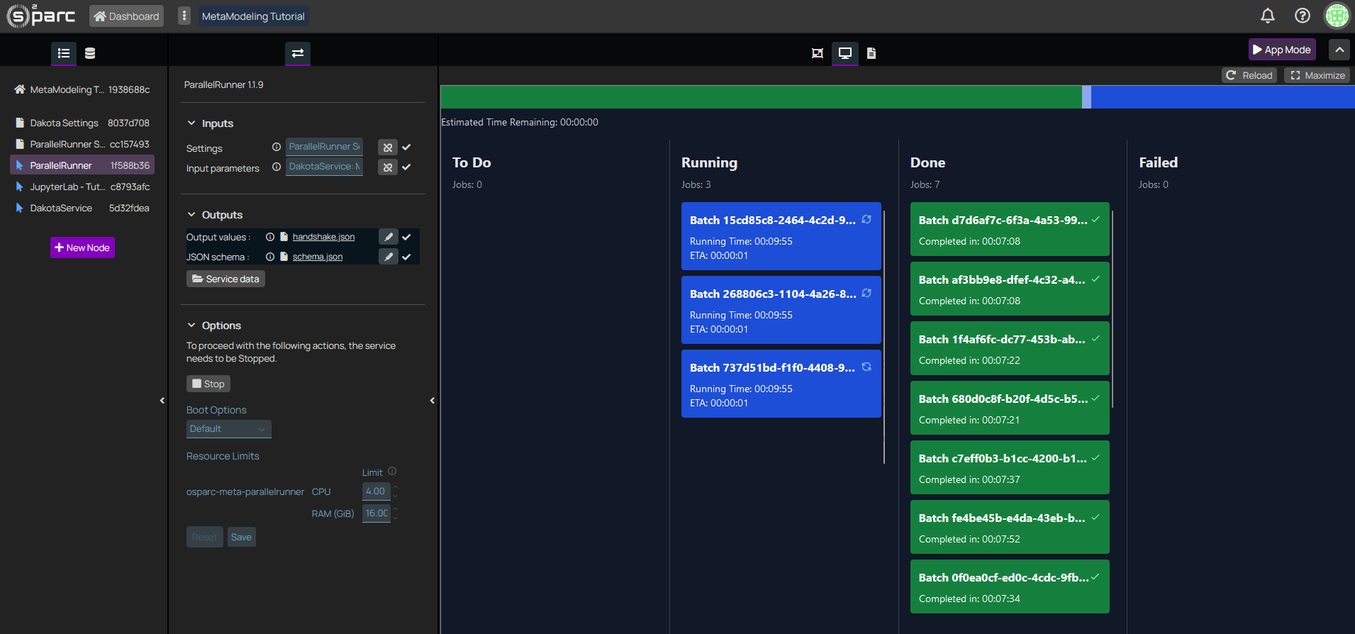
Figure 6: The interactive window of the ParallelRunner displays the status of the different jobs.
Current implementation stops ParallelRunner and DakotaService after a successful run. We are aware of this issue and working on a fix.
Loading & Visualizing results
Once all jobs have finished executing, the results file (results_eval.dat) will be available in the output folder of the DakotaService, which is connected to the inputs folder of the JupyterLab.
These results can be loaded through the commonly used Python's pandas package as a usual csv file (just note, the delimiter in Dakota files is a white space, not a comma). Let's display the activation (in terms of proportion of neural fibers activated) with respect to the input amplitude:
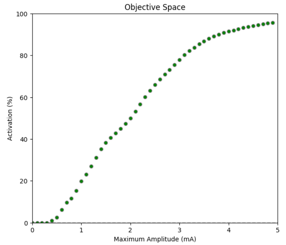
Figure 7: Proportion of neural fibers activated as a function of amplitude of the 0.3ms biphasic pulse
As expected, activation increases monotonically with stimulation amplitude. Low amplitudes produce no activation, the relationship is roughly linear for medium amplitudes (0.5 - 3.5mA), and starts reaching a plateau at higher amplitudes.
However, the relationship is not linear, as fibers are not homogeneously distributed in the anatomy, and a variety of fiber diameters are present (obtained from histological samples). Furthermore, it tends to plateau towards higher amplitudes.
Interpretation
These results are consistent with existing neuromodulation knowledge:
- There is a minimum stimulation threshold below which no fibers can be activated. Such threshold depends on implant location and shape, fiber types, tissue properties...
- The variety of fiber diameters and trajectories generates a variety of activation thresholds, resulting in a monotonic (and not necessarily linear) increase in activation with increasing stimulation intensity.
- There are fibers (far from the electrode, very small fiber diameter, or some geometrical / orientation configuration) which might be more difficult to activate, and thus the slope becomes smaller. Activating these fibers has a higher cost in terms of stimulation amplitude and specially in terms of energy consumption (which scales with the square of the amplitude). Furthermore, exposure safety must be considered. Therefore, complete activation of all fibers is often not pursued. Instead, the middle activation range is often sufficient to achieve clinical effects, and involves significantly lower safety and energy concerns.
Conclusions
This first part of the tutorial has shown how to run a series of pre-defined evaluations through the MetaModeling framework in o²S²PARC, in a scalable and reliable manner. Furthermore, results could be retrieved, analyzed and interpreted directly in the same notebook and service from which the execution was set up.
Current implementation stops ParallelRunner and DakotaService after a successful run. We are aware of this issue and working on a fix.Restarting the study (going back to the Dashboard and back into it) and re-executing the Setup cells is necessary, before executing Part 2. Please do that now.
Part 2 - LHS Sampling of the input space
In this section, we build up on the previous example to build up a sample of randomly-generated pulse shapes. Such sample can serve as an exploration of the input space (e.g. obtain correlation metrics between inputs and outputs) or as a basis to build a surrogate model (which can then be used for optimization or uncertainty quantification).
Sampling
The Latin Hypercube Sampling (LHS) algorithm is used to generate a sample. The LHS is a well-founded statistical algorithm which ensures data representativity (which is not guaranteed for a manually generated random sample) on N-dimensional spaces. Moreover, this method is available in Dakota and thus no additional coding effort or python packages are necessary.
The Dakota configuration file
Please inspect the new Dakota configuration file:
environment
    tabular_data
        tabular_data_file = 'results_sampling.dat'
    top_method_pointer = 'SAMPLING'

    method
        id_method = 'SAMPLING'
        sample_type
            lhs
        sampling
            samples = 500
            seed = 12345
        model_pointer = "EVALUATOR"

    model
        id_model = 'EVALUATOR'
        single
            interface_pointer = 'INTERFACE'
            variables_pointer = 'VARIABLES'
            responses_pointer = 'RESPONSES

    variables
        continuous_design = 9
        id_variables = 'VARIABLES'
            descriptors 'p1' 'p2' 'p3' 'p4' 'p5' 'p6' 'p7' 'p8' 'p9'
            lower_bounds      -5.0 -5.0 -5.0 -5.0 -5.0 -5.0 -5.0 -5.0 -5.0
            upper_bounds      5.0 5.0 5.0 5.0 5.0 5.0 5.0 5.0 5.0
    interface,
        id_interface = 'INTERFACE'
        batch
        python
            analysis_drivers
                'model'
    responses
        id_responses = 'RESPONSES'
        descriptors '1-activation' 'energy' 'maxamp'
        objective_functions = 3
        no_gradients
no_hessians- The main change is in the method section. Instead of a list_parameter_study, we have a lhs sampling algorithm with a given number of samples and a random seed (to ensure reproducibility).
- The other modification is at the variables - we must provide lower and upper bounds of the sampling.
- Everything else remains the same.
Executing Dakota
That's everything! Simply write the new configuration file to the output folder, and as before, head to the ParallelRunner interface to see the progress of your jobs.
Loading & Visualizing results
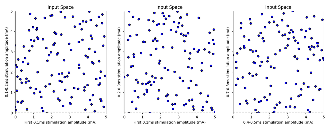
Figure 8: Latin Hypercube sample for multiple input variable pairs
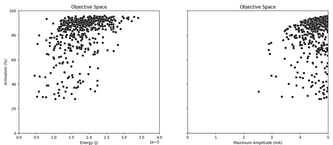
Figure 9: Neural fiber activation for the LH sample, represented against the two other output metrics: total energy and maximum amplitude.
Interpretation
The sample is well distributed in the input space (as expected from the Latin Hypercube Sampling algorithm). Note that this is a 9D distribution, and thus only projections to a lower dimensional can be visualized. These projections might exaggerate the closeness between certain pairs of points - the distance in all other dimensions is not being represented.
No samples managed to achieve very low activation, which is sensible given the results of the previous part - it is very unlikely that all randomized amplitudes between 0.0 and 5.0mA are below the 0.5-1mA value which marked low activation.
Furthermore, we see that the relationship is far from linear or monotonic - higher energy / maximal amplitude does not ensure higher activation. Thus, the interplay between parameters (in this case, the sequence along time of pulse amplitudes) must be playing a role - which justifies the next (and last) part of this tutorial: optimization.
Current implementation stops ParallelRunner and DakotaService after a successful run. We are aware of this issue and working on a fix.Restarting the study (going back to the Dashboard and back into it) and re-executing the Setup cells is necessary, before executing Part 3. Please do that now.
Part 3: Pulse Shape Optimization
The last part involves new elements from the MetaModeling field, namely surrogate-modeling and multi-objective optimization. There are a variety of online resources that might prove useful in expanding those concepts. This last part of the tutorial builds on that knowledge to illustrate the usefulness of these methods, and provides an example of more advanced MetaModeling workflows on o²S²PARC.
environment
    tabular_data
        tabular_data_file = 'results_optimization.dat'
    top_method_pointer = 'SUMO_OPT'

    method
        id_method = 'SUMO_OPT'
        surrogate_based_global
            model_pointer = 'SURR_MODEL'
            method_pointer = 'MOGA'
            max_iterations = 10

    model
        id_model 'SURR_MODEL'
        surrogate global
            gaussian_process surfpack


            dace_method_pointer = 'SAMPLING'"

    method
        id_method = 'MOGA'
        moga
        population_size = 32 # Set the initial population size in JEGA methods
        max_function_evaluations = 1000
        max_iterations = 100

        fitness_type
            layer_rank
        crossover_type
            multi_point_real 5
        mutation_type
            offset_uniform
        niching_type
            max_designs 32 # Limit number of solutions to remain in the population
        replacement_type
            elitist
        seed = 12345

    method
        id_method = 'SAMPLING'
        sample_type
            lhs
        sampling
            samples = 200
            seed = 12345
        model_pointer = "EVALUATOR"

    model
        id_model = 'EVALUATOR'
        single
            interface_pointer = 'INTERFACE'
            variables_pointer = 'VARIABLES'
            responses_pointer = 'RESPONSES'


    variables
        continuous_design = 9
        id_variables = 'VARIABLES'
            descriptors 'p1' 'p2' 'p3' 'p4' 'p5' 'p6' 'p7' 'p8' 'p9'
            lower_bounds      -5.0 -5.0 -5.0 -5.0 -5.0 -5.0 -5.0 -5.0 -5.0
            upper_bounds      5.0 5.0 5.0 5.0 5.0 5.0 5.0 5.0 5.0
    interface,
        id_interface = 'INTERFACE'
        batch
        python
            analysis_drivers
                'model'


    responses
        id_responses = 'RESPONSES'
        descriptors '1-activation' 'energy' 'maxamp'
        objective_functions = 3
        no_gradients
        no_hessians
There are several new elements on this workflow. The top level element is a surrogate-based optimizer method, which in turn is composed of two elements:
- Surrogate model: Based on the samples obtained from the true model (the evaluation pipeline), a Gaussian Process approximate model. This (meta)model aims to reproduce the input-output relationship of the underlying model at a much lower computational cost. Evaluations of the surrogate model happen inside Dakota and only take fractions of a second.
- MOGA optimizer: MOGA stands for Multi-Objective Genetic Algorithm. While the specifics of this optimization algorithm, and its parameters, are outside the scope of this tutorial, what matters is that this optimizer will be evaluated on the surrogate model, and thus performed very fast.
The surrogate-based optimizer is an iterative method: the optimal solution pool of the MOGA optimizer will be evaluated with the real model (the evaluation pipeline) and these results will make the surrogate model more accurate in the area of interest.
Loading & Visualizing result
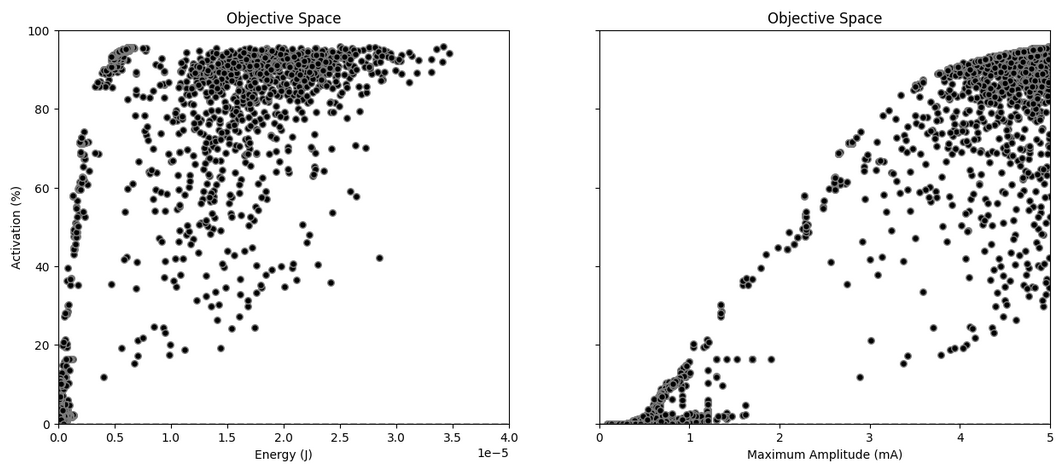
Figure 10: Optimization results. A well-defined Pareto front can be identified.
The results show a well identified Pareto front on the left side. Moreover, comparing with the LH sampling in the previous section, samples which are significantly more optimal have been identified. Let's inspect some of those:
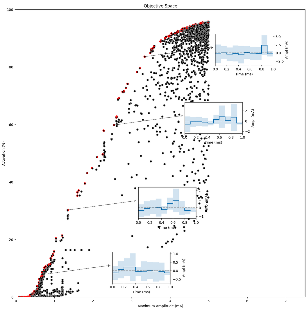
Figure 11: Pareto front and some identified solutions
Samples in red are Pareto-optimal - an improvement in activation is only possible at the cost of higher maximum amplitude; and a reduction of maximum amplitude will only come at the cost of reduced activation.
The insets show average (mean +- standard deviation) Pareto-optimal pulse shapes around that sample.
Interpretation
The optimizer seems to find it easier to focus on the high-activation regions, as well as in the low-activation region (below 20%). While the middle-activation area is not densely covered, there are samples all along this range which seem well aligned with the much more densely sampled Pareto front in the high- and low-intensity regions.
Inspecting the (average) samples at the Pareto front allows some trends can be identified:
- Ramp-up stimuli can be observed across the population, suggesting a more efficient energy usage.
- Most stimuli are composed of 1-2-3 consecutive sections of the same polarity, suggesting that 0.1-0.3ms stimulation is sufficient for this kind of fiber (myelinated). Thus, broader stimulation pulses are most likely sub-optimal in energy usage.
However, this analysis is hindered by the low density of samples in the mid-activation range. Could you do better? Maybe by changing the selection criteria of the genetic algorithm to encourage differentiation along the Pareto frontier? We refer the user to the radial niching type of the MOGA algorithm (instead of max_designs), and as an entry into the variety of options available - the possibilities are endless. Happy meta-modeling!
Conclusion
This tutorial introduces theoretical and practical aspects of MetaModeling, and applies them to a realistic clinical use case. Users have familiarized themselves with the o²S²PARC MetaModeling pipeline elements, Dakota input files, and visualization tools to represent these results, and had the chance to modify various parameters and observe the effects on results.
Advanced: Understanding the Runner template structure
While the Tutorial study above deals with the creation of samples and meta-modeling workflows, any meta-modeling application needs a base model.
As introduced above, the model in this tutorial will predict stimulation effects on neural fibers inside the sub-cutaneous nerves, based on pre-computed electric stimulation exposure data.
To be utilized in the Meta-Modeling framework, a Runner pipeline must be set up in o²S²PARC with the following characteristics:
- An empty FilePicker named "InputFile1".
- An output file probe which will receive a JSON file with the evaluation results.
- The evaluation pipeline itself. It can be comprised of data and any number of interconnected services, as long as they are all computational (see here for a more detailed explanation on computational pipelines).
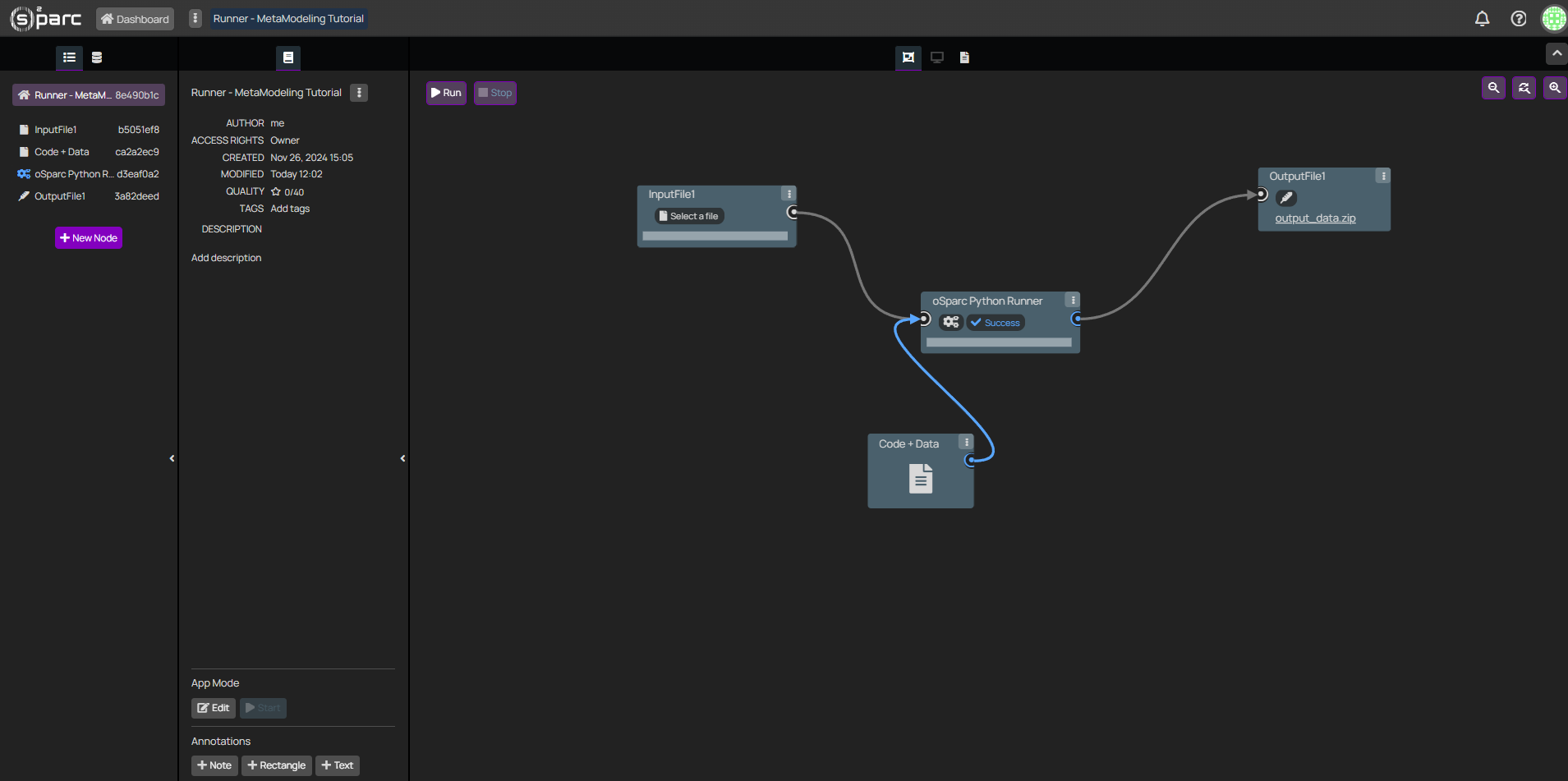
Runner computational pipeline to predict stimulation effects on sub-cutaneous nerves. This tutorial aims to keep it simple - nonetheless, an arbitrary number of inter-connected services can be provided, as long as the input-output structure is preserved.
Debugging the Runner pipeline
Please note that when evaluating the pipeline through the Meta-Modeling study, the logs of the pipeline will likely not be available, and thus it will be problematic to identify errors. Thus, it is strongly recommended to debug the pipeline manually.
Please follow the next steps:
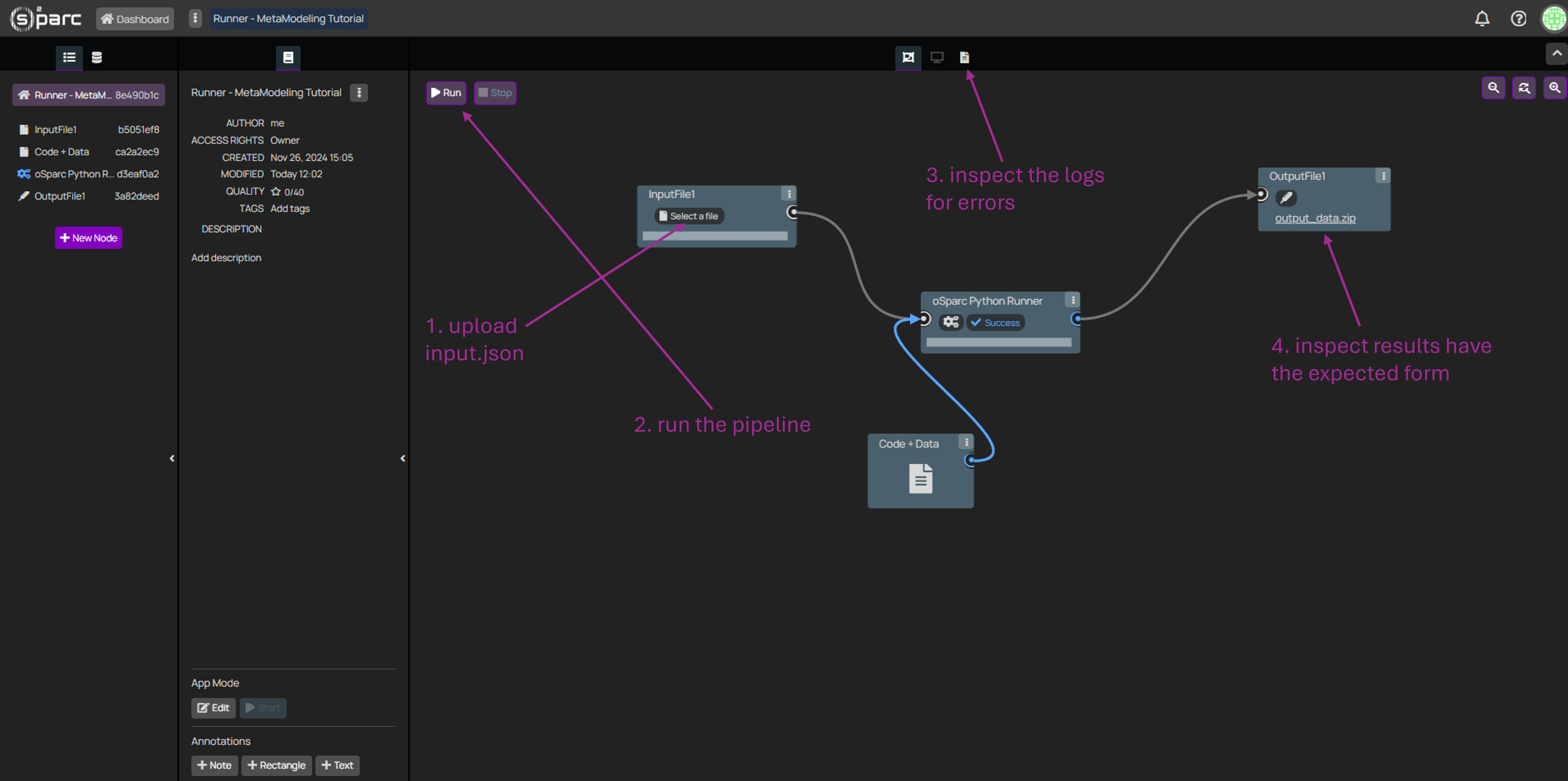
- Provide a manually created input JSON file, with the appropriate parameter keys (same that you will set up in the Meta-Modeling study), and suitable values.
- Click "Run" on the top-left corner.
- If an error arises anywhere in the pipeline, check the logs (top-center, third icon) in order to find more about the error. Iterate over steps 1-3 until the pipeline runs without errors.
- Once the pipeline runs without errors, inspect that the output produced has the expected form.
Once the Runner pipeline is ready, please close (and save) the study. Then, it must be published as a template in o²S²PARC:
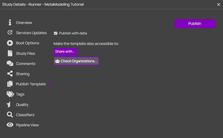
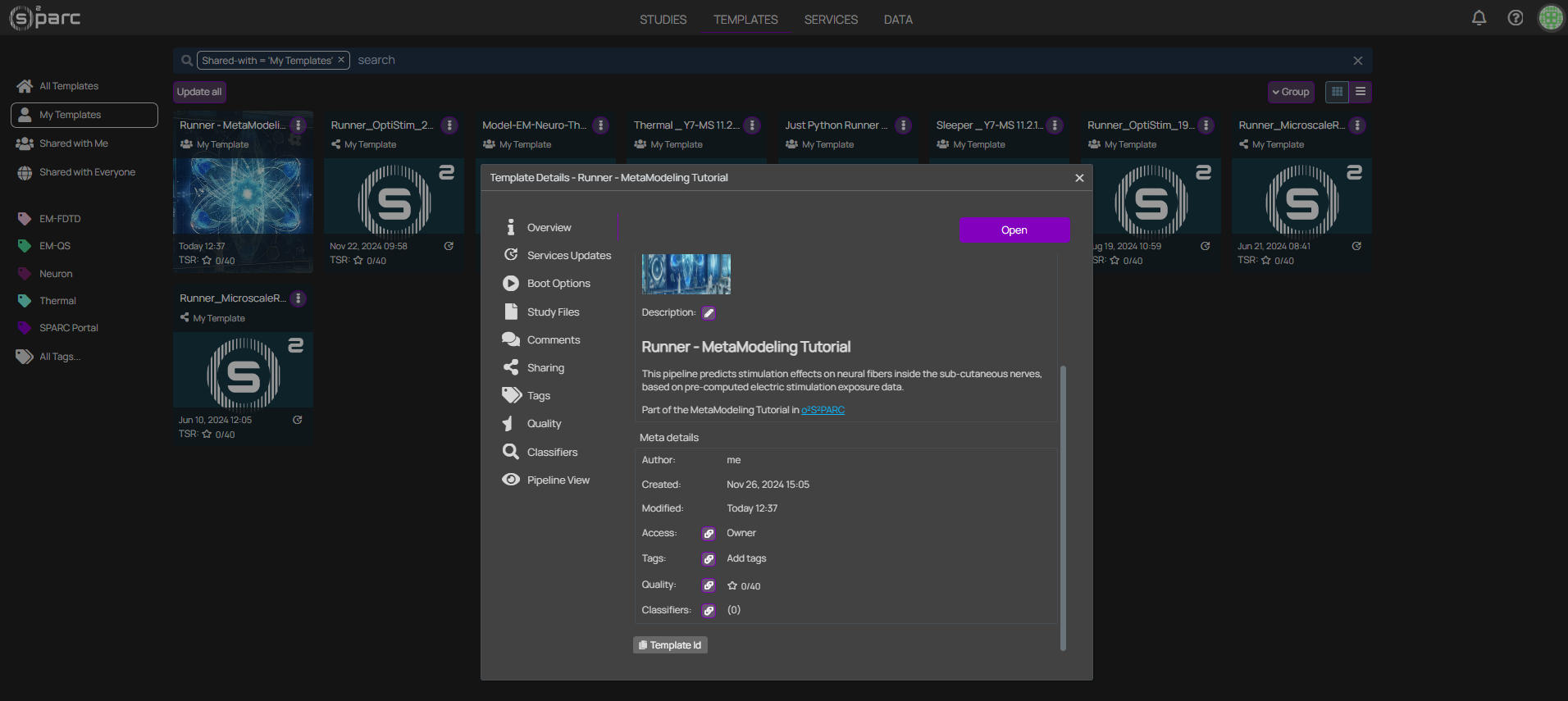
Once the publication process is finished (might take a few minutes), please head to the Templates section of o²S²PARC, select My Templates on the left menu, and click on the card of your published template. At the bottom of the Overview card, it is possible to copy the Template Id, which must be provided to the Parallel Runner through its settings.
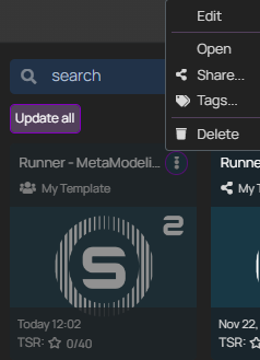
Tip: After publication, the template can still be edited by selecting Edit in the three dotted menu (see image). Note that normal opening of the template will generate a new study and thus changes made will not be saved in the template.
Advanced: Connecting the Services in a MetaModeling pipeline
If you want to set up your own MetaModeling pipeline, we recommend starting from a copy of the MetaModeling Tutorial template. Nonetheless, in case it becomes necessary, and to expand the knowledge of the users, this section will explain how to connect the different services in a MetaModeling pipeline.
- Output1 of the JupyterLab (to which dakota.in files will be copied) must be connected to input 1 (Dakota config) of the DakotaService.
- Output1 of the DakotaService (Dakota output files) must be connected back to the JupyterLab in order to retrieve the resulting .dat output files and analyze them. Moreover, this connection is necessary, as a back-and-forth handshake between the JupyterLab and the DakotaService is needed to establish a dynamic communication between both services.
- Output2 of the DakotaService (Map commands) must be forwarded to Input2 (Input parameters) of the ParallelRunner, which contains the parameter configurations to be run.
- Output1 of the ParallelRunner (Output values) must be connected back to Input2 of the DakotaService (Map feedback), thus closing the loop.
- Input3 of the DakotaService (Dakota service settings) and Input1 of the ParallelRunner (Settings) correspond to a JSON config file (these must be named settings.json). In the outputs of the these services you can find the JSON Schema output, which can be downloaded and inspected to see the options and values available.
Updated 8 months ago