Maps
An introduction and guide through the basics of the SPARC Portal maps
Maps on the SPARC Portal
The SPARC Portal displays detailed maps of the peripheral nervous system (PNS) based on SPARC data and information available in literature. These include the Anatomical Connectivity (AC) flatmaps, the Functional Connectivity (FC) flatmaps, and the Whole Body 3D map.
Explore the different maps in SPARC Apps (Figure 1).
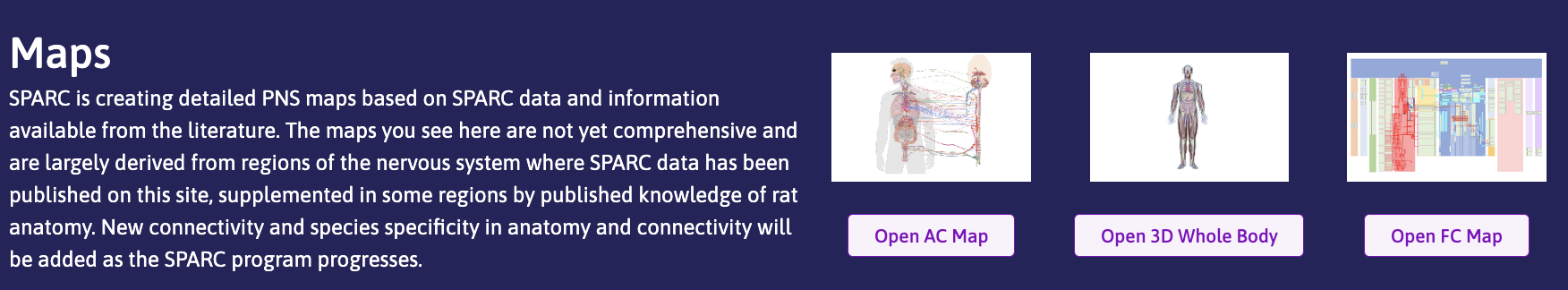
Figure 1: Switch between different types of Maps in SPARC Apps.
Flatmaps
Flatmaps published on the SPARC Portal provide 2D graphical representations of the anatomy, functionality, and topology of the connectivity of the PNS, in a Google Maps-like web-interface.
There are two types of flatmaps: an Anatomical Connectivity (AC) flatmap and a Functional Connectivity (FC) flatmap.
The AC and FC flatmaps allow knowledge captured in the SPARC Connectivity Knowledge base of the Autonomic Nervous system to be visualized and interactively explored on the SPARC Portal, including presenting relevant SPARC-published data as a user navigates through the interface.
The FC flatmap is a tool that provides the semantic description of all anatomical locations in the mammalian body along with the connectivity of networks that transfer information (neural connectivity) or mass flow (blood vessels and lymphatics) between these locations.
Learn more about Anatomical Connectivity (AC) and Functional Connectivity (FC) flatmaps.
Creating and displaying your own flatmapDetailed instructions on creating and displaying your own flatmaps are available on the Anatomical Flatmap Resources page.
Anatomical Models
3D Whole Body
The 3D whole-body map shows physical connectivity in an anatomically realistic context. Current developments are working toward enabling portal users to interactively explore connectivity seamlessly between the neuron population representation on the flatmaps and the nerve representation in the whole-body map.
Organ Scaffold Maps
Beyond the two-dimensional flatmaps, we also look to register data to three-dimensional organ scaffolds to provide maps in a common coordinate framework enabling disparate data to be integrated in order to improve our understanding of the collective SPARC knowledge. Learn more about Anatomical Models as datasets, how to explore them in the Scaffold Viewer, and how to map your data to existing scaffolds.
What can I do with Maps?
View anatomical features
Hovering over anatomical features will highlight it and prompt a tooltip with the feature ID. Clicking on these features will highlight it in green and outline it in red. Clicking the teardrop map marker will prompt the flatmap sidebar and provide all datasets and/or scaffolds relating to the selected feature. As seen in Figure 8, the liver has been selected and highlighted. Clicking the teardrop map marker prompts the flatmap sidebar with datasets relating to the liver. For more information, refer to the How to use the sidebar in Maps documentation.
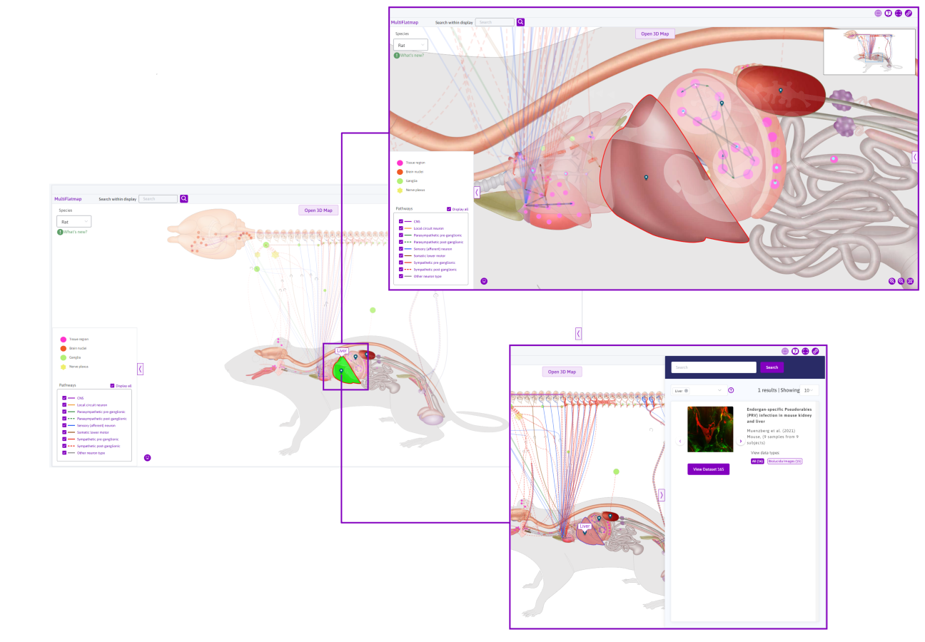
Figure 8: Selecting an anatomical structure (e.g. the Liver) on the rat flatmap.
View neuron pathways
In a similar manner, information on the neural pathways and other anatomical features can be observed. As seen in Figure 9, selecting the ‘Neruon type sdcol g’ pathway prompts a tooltip that provides more information. Scrolling down in the tooltip reveals a Search for data on components button, shown in Figure 10. This prompts related datasets in the flatmap sidebar.
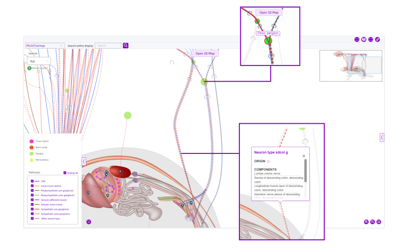
Figure 9: Selecting the pelvic ganglion highlights the feature and connected paths. Selecting the path ‘Neuron type sdcol g’ prompts a tooltip with further information.
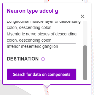
Figure 10: Scrolling down the tooltip that appears when selecting neuron pathways, a ‘Search for data on components’ button appears.
Similarly, in the FC map, information on the neural pathways can be observed by clicking on the desired pathway. Scrolling down reveals more information.
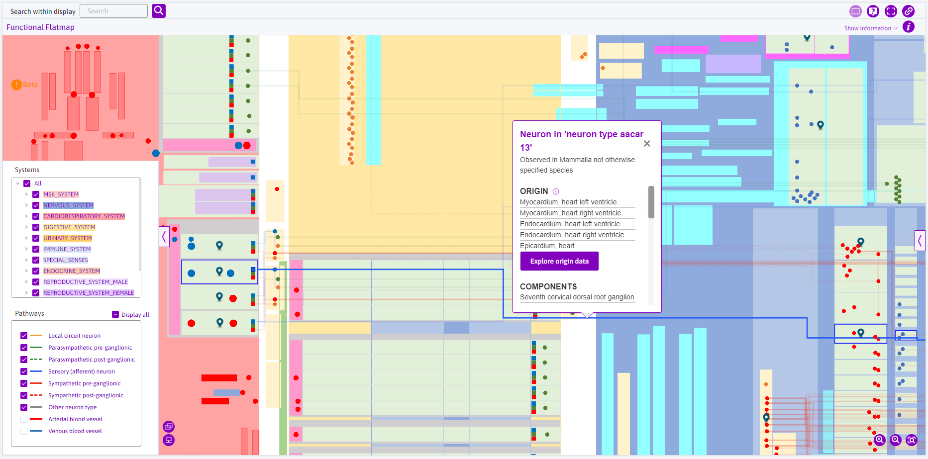
Figure 11: Selecting the neuron ‘aacar 13’ prompts the tooltip with information.
View scaffolds
In the AC flatmap, scaffolds can be viewed by clicking on the relevant anatomical features, like the urinary bladder. This will change the map interface to the ‘Bladder Scaffold 3D’ view.
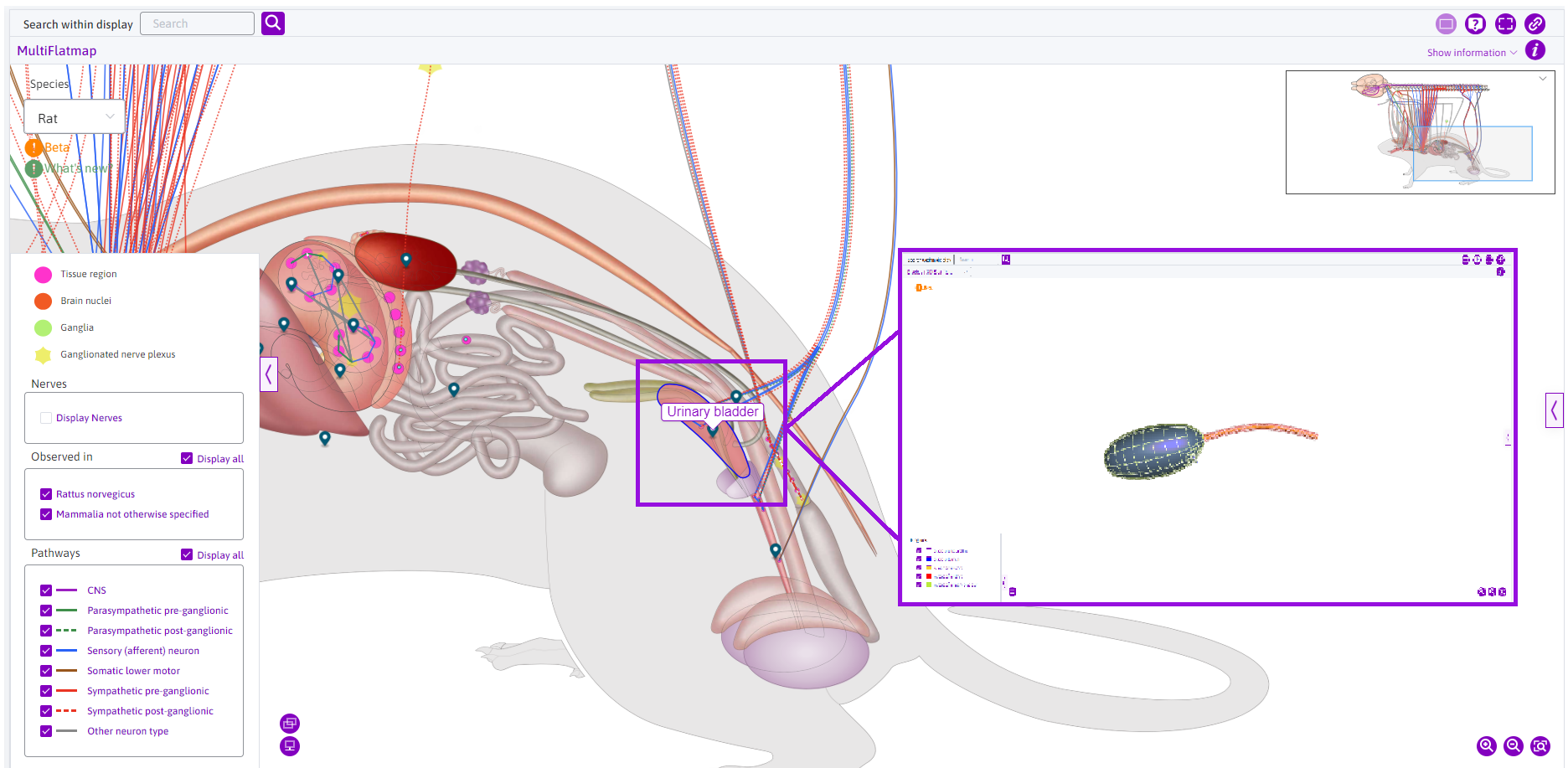
Figure 12: Clicking on anatomical features like the urinary bladder opens the scaffold of the organ.
Scaffolds can also be viewed by utilising the sidebar. Clicking on the chevron icon on the right, the sidebar can be opened. Scaffolds can be filtered by using the Data type category and choosing Scaffolds. Under any desired dataset, clicking on the Scaffolds tab allows a View Scaffold button. The View Scaffold button will prompt the corresponding scaffold in the display.
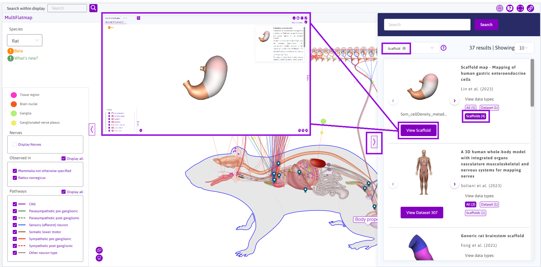
Figure 13: Accessing scaffolds via the sidebar by filtering datasets that involve scaffolds.
Accessing Maps
There are two ways to access Maps on the SPARC Portal (Figure 2). From the SPARC Portal homepage
- Click on the
View the Mapsbutton (1) to open Maps directly. By default, the integrated maps viewer shows a human male Flatmap. This is done using the flatmap viewer, from which anatomical scaffolds, data, and simulations can be accessed. Learn how to interact with the Integrated Maps Viewer. - Click on the SPARC Apps tab (2) from the top navigation bar
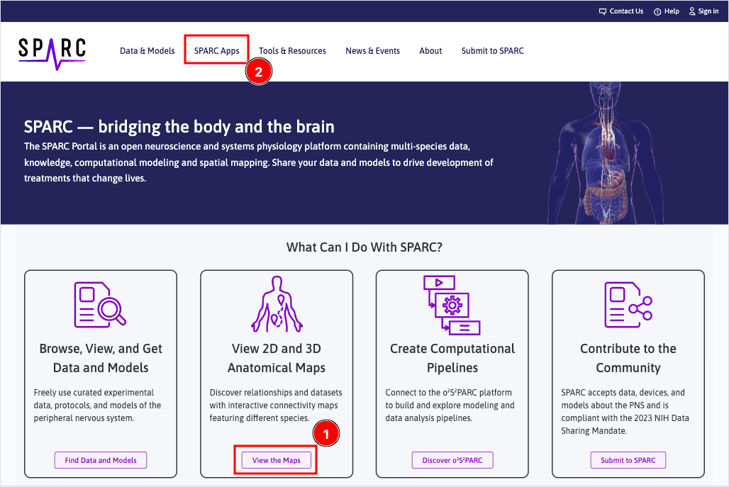
Figure 2: Accessing Maps from the SPARC Portal
From the SPARC Apps page (Figure 3):
- Click
View AC Mapto open the default Anatomical Connectivity flatmap (human male) or click the available species. - Click
View 3D Bodyto open the 3D whole-body scaffold. - Click
View FC Mapto open the Functional Connectivity flatmap.
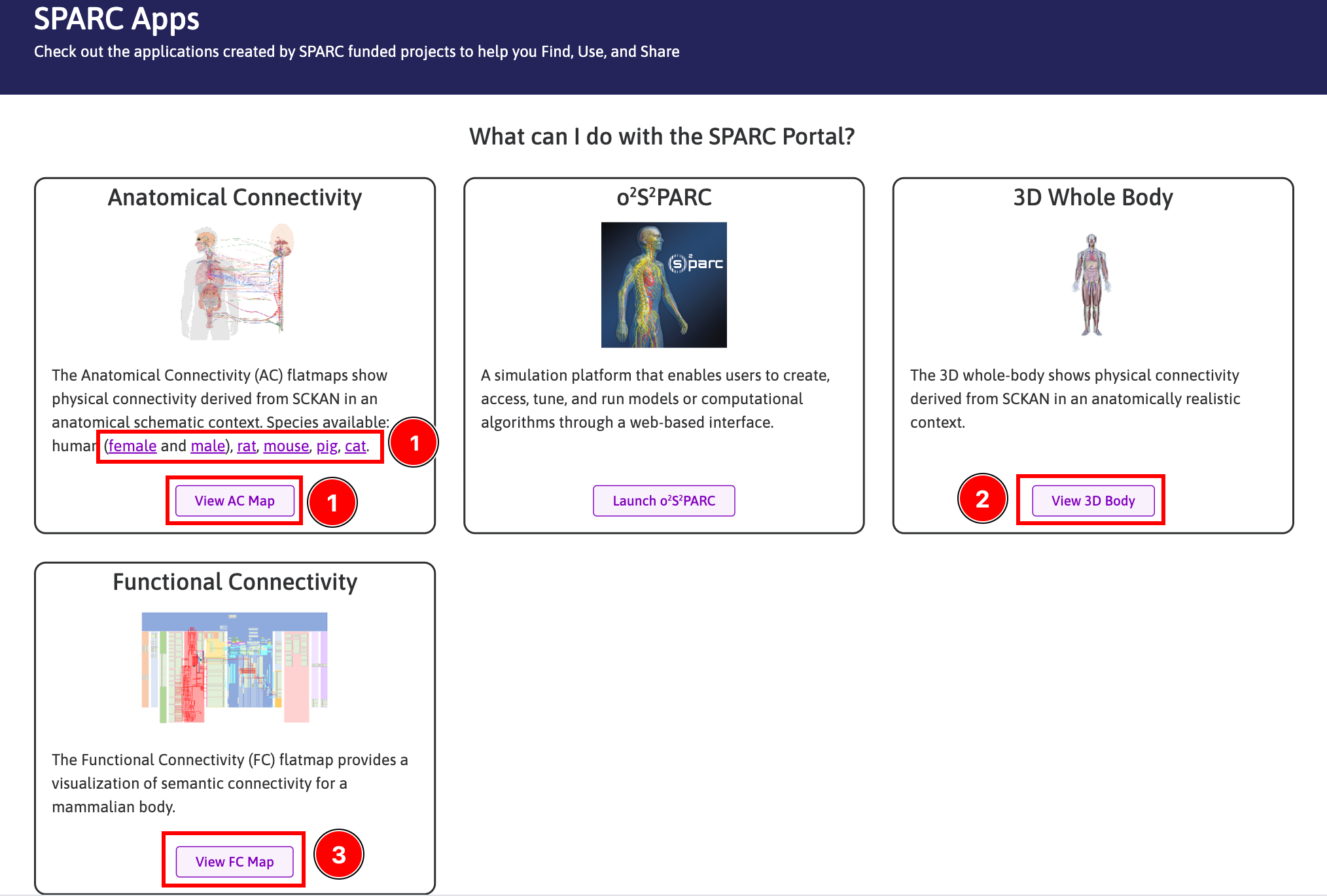
Figure 3: Accessing Maps from the SPARC Apps page
Updated 8 months ago